Page 127 - Distributed model predictive control for plant-wide systems

Local Cost Optimization-based Distributed Model Predictive Control 101

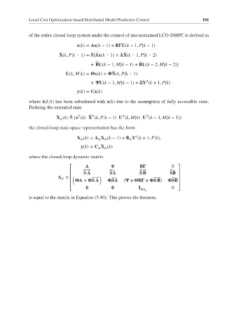
of the entire closed-loop system under the control of unconstrained LCO-DMPC is derived as
x(k)= Ax(k − 1)+ B U(k − 1, P|k − 1)

X(k, P|k − 1)= S[Ax(k − 1)+ AX(k − 1, P|k − 2)
̃ ̂
̂
+ BU(k − 1, M|k − 1)+ BU(k − 2, M|k − 2)]
̃
̂
U(k, M|k)= x(k)+ X(k, P|k − 1)
d
+ U(k − 1, M|k − 1)+ Y (k + 1, P|k)
y(k)= Cx(k)

where ̃ x(k|k) has been substituted with x(k) due to the assumption of fully accessible state.
Defining the extended state

̂ T
T
T
T
X (k) ≜ [x (k) X (k, P|k − 1) U (k, M|k) U (k − 1, M|k − 1)]
N
the closed-loop state-space representation has the form
d
X (k)= A X (k − 1)+ B Y (k + 1, P|k),
N
N
N
N
y(k)= C X (k)
N N
where the closed-loop dynamic matrix
A B
⎡ 0 ⎤
S A SA S B SB
⎢ ̃ ̃ ⎥
A = ⎢ ( ) ⎥
N ̃ ̃
⎢ A + S A SA ( + B + S B) SB⎥
⎢ ⎥
⎣ I Mn u 0 ⎦
is equal to the matrix in Equation (5.40). This proves the theorem.