Page 122 - Distributed model predictive control for plant-wide systems

96 Distributed Model Predictive Control for Plant-Wide Systems

⎡1.20e −27s 1.44e −27s ⎤
45s + 1 40s + 1
⎢ ⎥
⎢ −15s −15s ⎥
G (s)= ⎢ 1.52e 1.83e ⎥
d
25s + 1 20s + 1
⎢ ⎥
⎢ ⎥
1.44 1.26
⎢ ⎥
⎣ 27s + 1 32s + 1 ⎦
The main control objective of the whole system is to maintain the draw composition from the
top y and the side y of the column at specification (0.0 ± 0.005 at steady state). The constraints
1
2
of the output variables and the manipulated variables are set with |y | ≤ 0.5 (i = 1, 2), y ≥ 0.5
i
3
and |u | ≤ 0.5, |Δu | ≤ 0.2 (i = 1, 2, 3), respectively.
i
i
It can be seen that the Shell benchmark control problem is an extremely complex problem
which includes many possibly conflicting process requirements that are very difficult to sat-
isfy. The traditional QDMC algorithm utilized in the Shell benchmark control problem [97]
is computationally intensive, which not only increases the computational burden but is also
relatively difficult to implement. By examining the elements of G(s), it is observed that the
best pairing of manipulated and controlled variables is to control y with u , y with u , and y
1 1 2 2 3
with u . With the proposed distributed algorithm based on Nash optimality, first of all, divide
3
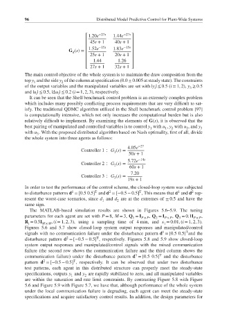
the whole system into three agents as follows:
4.05e −27
Controller 1 ∶ G (s)=
1
50s + 1
5.72e −14s
Controller 2 ∶ G (s)=
2
60s + 1
7.20
Controller 3 ∶ G (s)=
3
19s + 1
In order to test the performance of the control scheme, the closed-loop system was subjected
T
2
1
2
1
T
to disturbance patterns d = [0.5 0.5] and d = [−0.5 − 0.5] , This means that d and d rep-
resent the worst-case scenarios, since d and d are at the extremes of ± 0.5 and have the
1 2
same sign.
The MATLAB-based simulation results are shown in Figures 5.6–5.9. The tuning
parameters for each agent are set with P = 8, M = 3, Q = I , Q = I , Q = 0.1I ,
1 P × P 2 P × P 3 P × P
R = 0.5I ,(i = 1, 2, 3), using a sampling time of 4 min, and = 0.01, (i = 1, 2, 3).
i M × M i
Figures 5.6 and 5.7 show closed-loop system output responses and manipulated/control
1
T
signals with no communication failure under the disturbance pattern d = [0.5 0.5] and the
2
T
disturbance pattern d = [−0.5 − 0.5] , respectively. Figures 5.8 and 5.9 show closed-loop
system output responses and manipulated/control signals with the mixed communication
failure (the second row shows the communication failure and the third column shows the
1
T
communication failure) under the disturbance pattern d = [0.5 0.5] and the disturbance
2
T
pattern d = [−0.5 − 0.5] , respectively. It can be observed that under two disturbance
test patterns, each agent in this distributed structure can properly meet the steady-state
specifications, outputs y and y are rapidly stabilized to zero, and all manipulated variables
1
2
are within the saturation and rate limit constraints. By contrasting Figure 5.8 with Figure
5.6 and Figure 5.9 with Figure 5.7, we have that, although performance of the whole system
under the local communication failure is degrading, each agent can meet the steady-state
specifications and acquire satisfactory control results. In addition, the design parameters for