Page 147 - Distributed model predictive control for plant-wide systems

Cooperative Distributed Predictive Control 121

6.3.4 The Convergence Analysis of the Algorithm

The convergence is the key for an algorithm. Based on Equation (6.55), which is the whole sys-
tem control law, we can obtain the convergence condition for the DMPC based on plant-wide
optimality:
−1
[(D + R) D ] < 1 (6.56)
nd
d
where [⋅] is the spectrum radius of a matrix. If the algorithm is convergence, then we can
obtain the optimal control law without constraints:
l
Δu l+1 (k)= D [w(k)− y (k)] − D Δu (k) (6.57)
1
0
p0
M M
where
⎡D 11 ··· ⎤
⎢ D 11 ⋱ ⋮ ⎥
D = ⎢ ⋮ ⋱ ⋱ ⎥
1
⎣ ··· D mm ⎥
⎢
⎦
0 −D A
1m
11
⎡ 11 12 ··· −D A ⎤
⎢ −D A 21 0 ··· −D A ⎥
2m
22
22
D = ⎢ ⋮ ⋮ ⋱ ⋮ ⎥
1
⎢ ⎥
⎣−D mm A m1 −D mm A m2 ··· 0 ⎦
The control law mentioned in Equation (6.57) is not constricted to the optimal control law for
the centralized control. If the algorithm is convergence, from Equation (6.53), we can obtain
m m
∑ T ∗ ∗ ∑ T
A Q A Δu (k)+ R Δu (k)= A Q [w (k)− y (k)] (6.58)
ji j ji j,M i i,M ji j j j,p0
j=1 j=1
where Δu ∗ (k) and Δu ∗ (k) are the convergence values of the subsystems’ optimal control
i,M j,M
law at time k.
∗
Let Δu (k)=[Δu ∗ (k), … , Δu ∗ (k)], we can obtain a new form of the optimal control
M 1,M m,M
law
T
∗
T
−1
Δu (k)=(A QA + R) A Q[w(k)− y (k)] (6.59)
M p0
which is the same as Equation (6.42). That is to say that the algorithm mentioned in this section
is constricted to the optimal control law.
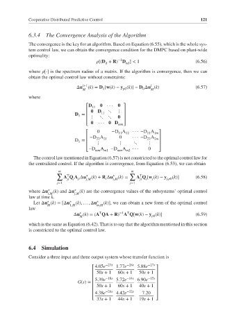
6.4 Simulation
Consider a three input and three output system whose transfer function is
4.05e −27s 1.77e −28s 5.88e −27s
⎡ ⎤
⎢ 50s + 1 60s + 1 50s + 1 ⎥
⎢ −18s −14s −15s ⎥
5.39e 5.72e 6.90e
G(s)= ⎢ ⎥
⎢ 50s + 1 60s + 1 40s + 1 ⎥
⎢ −20s −22s ⎥
⎢ 4.38e 4.42e 7.20 ⎥
33s + 1 44s + 1 19s + 1
⎣ ⎦