Page 217 - Distributed model predictive control for plant-wide systems

Cooperative Distributed Predictive Control with Constraints 191

Considering the limitation on the time consumption of communication, a stabilizing C-DMPC
design method, which communicates once a control period, is proposed in the next section.

9.3 Stabilizing Cooperative DMPC with Input Constraints

9.3.1 Formulation
In this section, m separate optimal control problems, one for each subsystem and the C-DMPC
algorithm with communicating once a control period, is defined. In every distributed optimal
control problem, the same constant prediction horizon N, N > 1, is used. And every distributed
MPC law is updated globally synchronously. At each update, every subsystem-based MPC
optimizes only for its own open-loop control sequence, given the current states and the esti-
mated inputs of the whole system.
To proceed, we need the following assumption, and we also define the necessary notations
in Table 9.1.
Assumption 9.1 For every subsystem i ∈ P there exists a state feedback u = K x such that
i
i
the closed-loop system x(k + 1) = A x(k) is asymptotically stable, where A = A + BK and
c
c
K = block-diag(K , K , … , K ).
2
1
m
The state evolution of subsystem S , j ∈ P , is affected by the optimal control decision of
j −i
S , and the affection on the control performance of subsystem S may be negative sometime.
i j
Thus, the idea of global cost optimization [114] is adopted here, that is, each subsystem-based
MPC takes the cost function of all subsystems into account; more specifically, the performance
index is defined as
N−1 ( )
∑
J = ‖̂ x (k + N|k, i)‖ + ‖̂ x (k + l|k, i)‖ + u (k + l|k) ‖
‖
i P Q ‖ i ‖R j
l=0
T
T
T
where Q = Q > 0, R = R > 0, P = P > 0. And the matrix P is chosen to satisfy the
j
j
Lyapunov equation
T
̂
A PA − P =−Q
c
c
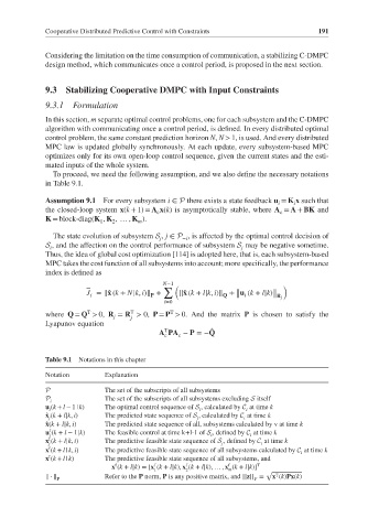
Table 9.1 Notations in this chapter
Notation Explanation
P The set of the subscripts of all subsystems
P The set of the subscripts of all subsystems excluding S itself
i
u (k + l − 1| k) The optimal control sequence of S , calculated by C at time k
i i i
̂ x (k + l|k, i) The predicted state sequence of S , calculated by C at time k
j j i
̂ x(k + l|k, i) The predicted state sequence of all, subsystems calculated by v at time k
f
u (k + l − 1|k) The feasible control at time k+l-1 of S ,definedby C at time k
i i i
f
x (k + l|k, i) The predictive feasible state sequence of S ,definedby C at time k
j j i
f
x (k + l | k, i) The predictive feasible state sequence of all subsystems calculated by C at time k
i
f
x (k + l | k) The predictive feasible state sequence of all subsystems, and
f
f
f
f
x (k + l|k)=[x (k + l|k), x (k + l|k), … , x (k + l|k)] T
1 2 m √
T
‖ ⋅ ‖ P Refer to the P norm, P is any positive matrix, and ||z|| = x (k)Px(k)
P