Page 313 - Distributed model predictive control for plant-wide systems

Operation Optimization of Multitype Cooling Source System Based on DMPC 287

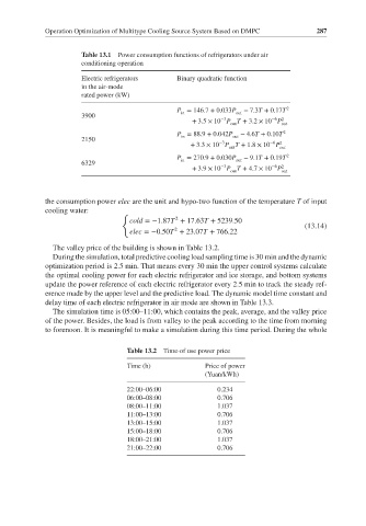
Table 13.1 Power consumption functions of refrigerators under air
conditioning operation
Electric refrigerators Binary quadratic function
in the air-mode
rated power (kW)

P = 146.7 + 0.033P out − 7.3T + 0.17T 2
in
3900
−3
−6
+ 3.5 × 10 P T + 3.2 × 10 P 2 out
out
P = 88.9 + 0.042P out − 4.6T + 0.10T 2
in
2150
−3
−6
+ 3.3 × 10 P T + 1.8 × 10 P 2 out
out
P = 270.9 + 0.030P out − 9.1T + 0.19T 2
in
6329
−3
−6
+ 3.9 × 10 P T + 4.7 × 10 P 2 out
out
the consumption power elec are the unit and hypo-two function of the temperature T of input
cooling water:
{
2
cold =−1.87T + 17.63T + 5239.50
(13.14)
2
elec =−0.50T + 23.07T + 766.22
The valley price of the building is shown in Table 13.2.
During the simulation, total predictive cooling load sampling time is 30 min and the dynamic
optimization period is 2.5 min. That means every 30 min the upper control systems calculate
the optimal cooling power for each electric refrigerator and ice storage, and bottom systems
update the power reference of each electric refrigerator every 2.5 min to track the steady ref-
erence made by the upper level and the predictive load. The dynamic model time constant and
delay time of each electric refrigerator in air mode are shown in Table 13.3.
The simulation time is 05:00–11:00, which contains the peak, average, and the valley price
of the power. Besides, the load is from valley to the peak according to the time from morning
to forenoon. It is meaningful to make a simulation during this time period. During the whole
Table 13.2 Time-of use power price

Time (h) Price of power
(Yuan/kWh)

22:00–06:00 0.234
06:00–08:00 0.706
08:00–11:00 1.037
11:00–13:00 0.706
13:00–15:00 1.037
15:00–18:00 0.706
18:00–21:00 1.037
21:00–22:00 0.706