Page 311 - Distributed model predictive control for plant-wide systems

Operation Optimization of Multitype Cooling Source System Based on DMPC 285

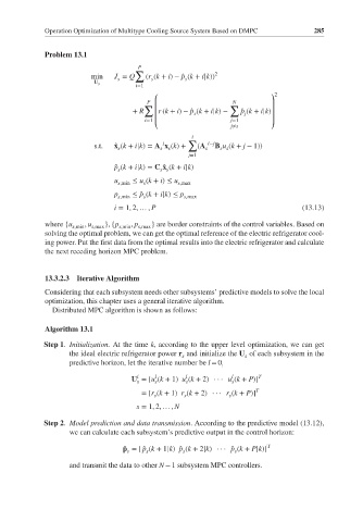
Problem 13.1
P
∑ 2
min J = Q (r (k + i)− ̂p (k + i|k))
s s s
U s
i=1
2
P ⎛ N ⎞
∑ ⎜ ∑ ⎟
+ R ⎜ (k + i) − ̂p (k + i|k)− ̂ p (k + i|k) ⎟
r
j
s
i=1 ⎜ j=1 ⎟
⎝ j≠s ⎠
i
∑ i−j
i
s.t. ̂ x (k + i|k)= A x (k)+ (A B u (k + j − 1))
s s s s s s
j=1
̂ p (k + i|k)= C ̂ x (k + i|k)
s s s
u s,min ≤ u (k + i) ≤ u s,max
s
p s,min ≤ ̂p (k + i|k) ≤ p s,max
s
i = 1, 2, … , P (13.13)
where {u s,min , u s,max }, {p s,min , p s,max } are border constraints of the control variables. Based on
solving the optimal problem, we can get the optimal reference of the electric refrigerator cool-
ing power. Put the first data from the optimal results into the electric refrigerator and calculate
the next receding horizon MPC problem.

13.3.2.3 Iterative Algorithm
Considering that each subsystem needs other subsystems’ predictive models to solve the local
optimization, this chapter uses a general iterative algorithm.
Distributed MPC algorithm is shown as follows:

Algorithm 13.1
Step 1. Initialization. At the time k, according to the upper level optimization, we can get
the ideal electric refrigerator power r and initialize the U of each subsystem in the
s
s
predictive horizon, let the iterative number be l = 0 :
l
l
l
l
U =[u (k + 1) u (k + 2)· · · u (k + P)] T
s
s
s
s
=[r (k + 1) r (k + 2)· · · r (k + P)] T
s s s
s = 1, 2, … , N
Step 2. Model prediction and data transmission. According to the predictive model (13.12),
we can calculate each subsystem’s predictive output in the control horizon:
̂ p =[ ̂p (k + 1|k) ̂p (k + 2|k)· · · ̂p (k + P|k)] T
s
s
s
s
and transmit the data to other N − 1 subsystem MPC controllers.