Page 68 - Dynamic Vision for Perception and Control of Motion

52 2 Basic Relations: Image Sequences – “the World”

for the linearized perturbation system follows:
dx / dt F x ˜ ' v t() , (2.30)
with F df / dX N (2.31)
as an (n × n)-matrix and v’(t) an additive noise term.

2.2.5.2 Transition Matrices for Single Step Predictions
Equation 2.30 with matrix F may be transformed into a difference equation with
cycle time T for grid point spacing by one of the standard methods in systems dy-
namics or control engineering. (Precise numerical integration from 0 to T for v = 0
may be the most convenient one for complex right–hand sides.) The resulting gen-
eral form then is

x [(k 1) ] T A ˜ [ x kT ] v [kT ]
(2.32)
or in short-hand x k 1 Ax ˜ k v ,
k
with matrix A of the same dimension as F. In the general case of local lineariza-
tion, all entries of this matrix may depend on the nominal state variables. Proce-
dures for computing the elements of matrix A from F have to be part of the 4-D
knowledge base for the application at hand.
For objects, the trajectory is fixed by the initial conditions and the perturbations
encountered. For subjects having additional control terms in these equations, de-
termination of the actual control output may be a rather involved procedure. The
wide variety of subjects is discussed in Chapter 3.

2.2.5.3 Basic Dynamic Model: Decoupled Newtonian Motion

The most simple and yet realistic dynamic model for the motion of a rigid body
under external forces F e is the Newtonian law
²/ dt 6
t
dx ² F e ( ) / m . (2.33)
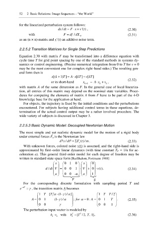
With unknown forces, colored noise v(t) is assumed, and the right–hand side is
approximated by first–order linear dynamics (with time constant T C = 1/Į for ac-
celeration a). This general third-order model for each degree of freedom may be
written in standard state space form [BarShalom, Fortmann 1988]
§· § 01 0 · § · § ·
x
0
x
¨¸ ¨ ¸ ¨ ¸ ¨ ¸
ddt V / 0 0 1 ˜ V 0 v t ().˜ (2.34)
¨¸ ¨ ¸ ¨ ¸ ¨ ¸
¨¸ ¨ ¸ ¨ ¸ ¨ ¸
a
1
a
©¹ © 00 -Į ¹ © ¹ © ¹
F g
For the corresponding discrete formulation with sampling period T and
D
e - T J , the transition matrix A becomes
§ 1 T [T D -(1- ) / ]· D § J 1 T T / 2·
¨ ¸ ¨ ¸
A 01 (1- ) / D ; for D 0: A 01 T . (2.35)
J
¨ ¸ 0 ¨ ¸
¨ ¸ ¨ ¸
© 0 0 J ¹ © 0 0 1 ¹
The perturbation input vector is modeled by
˜
T
bv k with b T k [T 2 /2, , 1] , (2.36)
k