Page 312 - Dynamics and Control of Nuclear Reactors

314 APPENDIX F State variable models and transient analysis

y

y4

y3
y2

y1
y0

x0 x1 x2 x3 x4 x
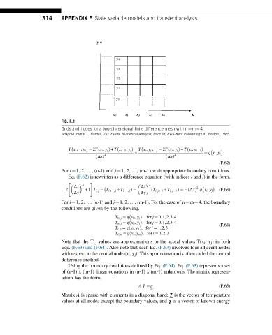
FIG. F.1
Grids and nodes for a two-dimensional finite difference mesh with n¼m¼4.
Adapted from R.L. Burden, J.D. Faires, Numerical Analysis, third ed, PWS-Kent Publishing Co., Boston, 1985.

Tx i +1 , y j 2Tx i , y j + Tx i 1 , y j Tx i , y j +1 2Tx i , y j + Tx i , y j 1
+
2 2 ¼ qx i , y j
ð ΔxÞ ð ΔyÞ
(F.62)
For i¼1, 2, …, (n-1) and j¼1, 2, …, (m-1) with appropriate boundary conditions.
Eq. (F.62) is rewritten as a difference equation (with indices i and j) in the form.
" #
2 2
Δx Δx 2
2 +1 T i, j T i +1, j + T i 1, j T i, j +1 + T i, j 1 ¼ Δxð Þ qx i , y j (F.63)
Δy Δy
For i¼1, 2, …, (n-1) and j¼1, 2, …, (m-1). For the case of n¼m¼4, the boundary
conditions are given by the following.

T 0, j ¼ gx 0 , y j , forj ¼ 0,1,2,3,4

T n, j ¼ gx n , y j , forj ¼ 0,1,2,3,4
(F.64)
T i,0 ¼ gx i , y 0 Þ, fori ¼ 1,2,3
ð
T i,m ¼ gx i , y m Þ, fori ¼ 1,2,3
ð
Note that the T i,j values are approximations to the actual values T(x i ,y j ) in both
Eqs. (F.63) and (F.64). Also note that each Eq. (F.63) involves four adjacent nodes
with respect to the central node (x i ,y j ). This approximation is often called the central
difference method.
Using the boundary conditions defined by Eq. (F.64), Eq. (F.63) represents a set
of (n-1) x (m-1) linear equations in (n-1) x (m-1) unknowns. The matrix represen-
tation has the form.
A T ¼ q (F.65)

Matrix A is sparse with elements in a diagonal band; T is the vector of temperature
values at all nodes except the boundary values, and q is a vector of known energy