Page 309 - Dynamics and Control of Nuclear Reactors

APPENDIX F State variable models and transient analysis 311

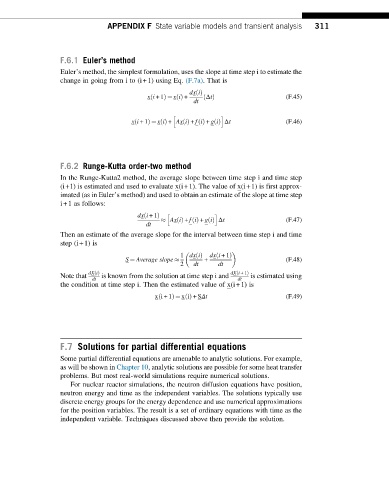
F.6.1 Euler’s method
Euler’s method, the simplest formulation, uses the slope at time step i to estimate the
change in going from i to (i+1) using Eq. (F.7a). That is
dxiðÞ
Δt
xi +1Þ ¼ xiðÞ + ðÞ (F.45)
ð
dt
h i
xi +1Þ ¼ xi ðÞ + Axi ðÞ + fi ðÞ + gi ðÞ Δt (F.46)
ð

F.6.2 Runge-Kutta order-two method
In the Runge-Kutta2 method, the average slope between time step i and time step
(i+1) is estimated and used to evaluate x(i+1). The value of x(i+1) is first approx-
imated (as in Euler’s method) and used to obtain an estimate of the slope at time step
i+1 as follows:
ð
dxi +1Þ h i
AxiðÞ + fiðÞ + giðÞ Δt (F.47)
dt
Then an estimate of the average slope for the interval between time step i and time
step (i+1) is

ð
1 dxiðÞ dxi +1Þ
S ¼ Average slope + (F.48)
2 dt dt
ð
Note that dx iðÞ is known from the solution at time step i and dx i +1Þ is estimated using
dt dt
the condition at time step i. Then the estimated value of x(i+1) is
xi + 1Þ ¼ xiðÞ + SΔt (F.49)
ð

F.7 Solutions for partial differential equations

Some partial differential equations are amenable to analytic solutions. For example,
as will be shown in Chapter 10, analytic solutions are possible for some heat transfer
problems. But most real-world simulations require numerical solutions.
For nuclear reactor simulations, the neutron diffusion equations have position,
neutron energy and time as the independent variables. The solutions typically use
discrete energy groups for the energy dependence and use numerical approximations
for the position variables. The result is a set of ordinary equations with time as the
independent variable. Techniques discussed above then provide the solution.