Page 304 - Dynamics and Control of Nuclear Reactors

306 APPENDIX F State variable models and transient analysis

or
dx
¼ AxtðÞ + BftðÞ
dt
This is the original set of differential equations.
The state transition matrix φ(t)¼exp(At) also has the following properties.
ðÞφ t 2 ¼ φ t 1 + t 2 Þ
φ t 1 ðÞ ð (F.31)
1
ð
φ tðÞ ¼ φ tÞ (F.32)
ð t
xtðÞ ¼ φ t t 0 Þxt 0 + φ t τÞBf τðÞdτ (F.33)
ð
ð
ðÞ
t 0

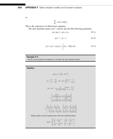
Example F.3
For the system defined in Example F.2, determine the state transition matrix.

Solution

h i
φ tðÞ ¼ L 1 ð sI AÞ 1

2 3 s +2 3
A ¼ , ð sI AÞ ¼
1 4 1 s +4
1 s +4 3
1
ð sI AÞ ¼
ð s +1Þ s +5Þ 1 s +2
ð
2 3
s +4 3
ð
ð
ð s +1Þ s +5Þ s +1Þ s +5Þ
ð
6 7
¼ 6 1 s +2 7
4 5
ð
ð
ð
ð s +1Þ s +5Þ s +1Þ s +5Þ
2 3
3 1 1 1 3 1 3 1
+ +
ð
ð
4 s +1Þ 4 s +5Þ 4 s +1Þ 4 s +5Þ
ð
ð
6 7
¼ 6 7
1 1 1 1 1 1 3 1
4 5
+ +
ð
ð
ð
ð
4 s +1Þ 4 s +5Þ 4 s +1Þ 4 s +5Þ
Taking Laplace inverse transform gives the state transition matrix.
2 3
3 1 3 3
t
t
e + e 5t e + e 5t
4 4 4 4
6 7
φ tðÞ ¼ 4 1 1 1 3 5
t
t
e + e 5t e + 3 5t
4 4 4 4