Page 305 - Dynamics and Control of Nuclear Reactors

APPENDIX F State variable models and transient analysis 307

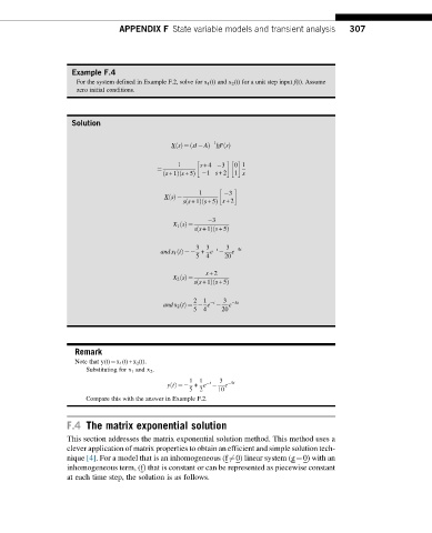
Example F.4
For the system defined in Example F.2, solve for x 1 (t) and x 2 (t) for a unit step input f(t). Assume
zero initial conditions.

Solution

1
ð
XsðÞ ¼ sI AÞ bF sðÞ
0 1
1 s +4 3
¼
ð s +1Þ s +5Þ 1 s +2 1 s
ð
1 3
XsðÞ ¼
ss +1Þ s +5Þ s +2
ð
ð
3
X 1 sðÞ ¼
ð
ss +1Þ s +5Þ
ð
3 3 t 3 5t
and x 1 tðÞ ¼ + e e
5 4 20
s +2
X 2 sðÞ ¼
ss +1Þ s +5Þ
ð
ð
2 1 3
t
and x 2 tðÞ ¼ e e 5t
5 4 20

Remark
Note that y(t)¼x 1 (t)+x 2 (t).
Substituting for x 1 and x 2 .
1 1 3
t
ytðÞ ¼ + e e 5t
5 2 10
Compare this with the answer in Example F.2.

F.4 The matrix exponential solution
This section addresses the matrix exponential solution method. This method uses a
clever application of matrix properties to obtain an efficient and simple solution tech-
nique [4]. For a model that is an inhomogeneous (f6¼0) linear system (g¼0) with an
inhomogeneous term, (f) that is constant or can be represented as piecewise constant
at each time step, the solution is as follows.