Page 50 - Dynamics and Control of Nuclear Reactors

4.6 Sinusoidal reactivity and frequency response 41

2.5

2

1.5
P/P(0)
1

0.5
Exact solution
Perturbation solution
0
0 10 20 30 40 50 60
Time (s)
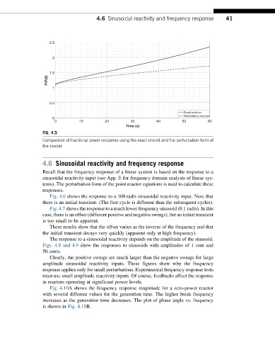
FIG. 4.5
Comparison of fractional power response using the exact model and the perturbation form of
the model.

4.6 Sinusoidal reactivity and frequency response

Recall that the frequency response of a linear system is based on the response to a
sinusoidal reactivity input (see App. E for frequency domain analysis of linear sys-
tems). The perturbation form of the point reactor equations is used to calculate these
responses.
Fig. 4.6 shows the response to a 100 rad/s sinusoidal reactivity input. Note that
there is an initial transient. (The first cycle is different than the subsequent cycles).
Fig. 4.7 shows the response to a much lower frequency sinusoid (0.1 rad/s). In this
case, there is an offset (different positive and negative swings), but an initial transient
is too small to be apparent.
These results show that the offset varies as the inverse of the frequency and that
the initial transient decays very quickly (apparent only at high frequency).
The response to a sinusoidal reactivity depends on the amplitude of the sinusoid.
Figs. 4.8 and 4.9 show the responses to sinusoids with amplitudes of 1 cent and
50 cents.
Clearly, the positive swings are much larger than the negative swings for large
amplitude sinusoidal reactivity inputs. These figures show why the frequency
response applies only for small perturbations. Experimental frequency response tests
must use small amplitude reactivity inputs. Of course, feedbacks affect the response
in reactors operating at significant power levels.
Fig. 4.10A shows the frequency response magnitude for a zero-power reactor
with several different values for the generation time. The higher break frequency
increases as the generation time decreases. The plot of phase angle vs. frequency
is shown in Fig. 4.10B.