Page 227 - Dynamics of Mechanical Systems

0593_C07_fm Page 208 Monday, May 6, 2002 2:42 PM

208 Dynamics of Mechanical Systems

S
n a

G
O
P
G

d = | P × N |
G a
d
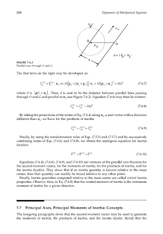
FIGURE 7.6.2
Parallel axes through O and G.
The first term on the right may be developed as:

[
2
×
I GO = I GO ⋅n == M p G (n × p G)] ⋅n = M(p × n a) = Md 2 (7.6.7)
aa a a a a G
where d is pG × n . Then, d is seen to be the distance between parallel lines passing
a
through O and G and parallel to n (see Figure 7.6.2). Equation (7.6.6) may then be written:
a
I SO = I SG + Md 2 (7.6.8)
aa aa
By taking the projections of the terms of Eq. (7.6.4) along n , a unit vector with a direction
b
different than n , we have for the products of inertia:
a
I SO = I GO + I SG (7.6.9)
ab ab ab
Finally, by using the transformation rules of Eqs. (7.5.5) and (7.5.7) and by successively
combining terms of Eqs. (7.6.6) and (7.6.8), we obtain the analogous equation for inertia
dyadics:

I SO = I G O + I S G (7.6.10)

Equations (7.6.4), (7.6.6), (7.6.9), and (7.6.10) are versions of the parallel axis theorem for
the second-moment vector, for the moments of inertia, for the products of inertia, and for
the inertia dyadics. They show that if an inertia quantity is known relative to the mass
center, then that quantity can readily be found relative to any other point.
Finally, inertia quantities computed relative to the mass center are called central inertia
properties. Observe, then, in Eq. (7.6.8) that the central moment of inertia is the minimum
moment of inertia for a given direction.

7.7 Principal Axes, Principal Moments of Inertia: Concepts

The foregoing paragraphs show that the second-moment vector may be used to generate
the moments of inertia, the products of inertia, and the inertia dyadic. Recall that the