Page 377 - Dynamics of Mechanical Systems

0593_C11_fm Page 358 Monday, May 6, 2002 2:59 PM

358 Dynamics of Mechanical Systems

Z
n
3 N 3
θ
D n 2
Ψ
G
X
φ Y
N 1
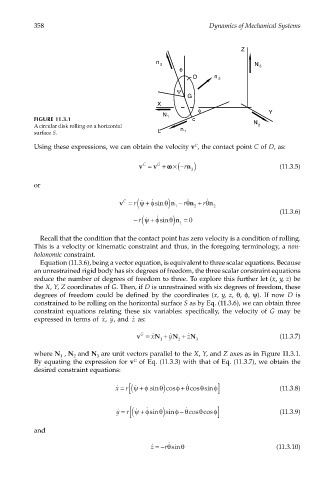
FIGURE 11.3.1 c N
A circular disk rolling on a horizontal n 2
surface S. L 1

C
Using these expressions, we can obtain the velocity v , the contact point C of D, as:
v = v + ωω × n r − ( ) (11.3.5)
C
G
3
or

v = ( ψφ ˙ n ) θ − rθ ˙ n + rθ ˙ n
C
r ˙
+ sin
1 2 2
(11.3.6)
− r( ψφ ˙ n ) θ = 0
˙
+ sin
1
Recall that the condition that the contact point has zero velocity is a condition of rolling.
This is a velocity or kinematic constraint and thus, in the foregoing terminology, a non-
holonomic constraint.
Equation (11.3.6), being a vector equation, is equivalent to three scalar equations. Because
an unrestrained rigid body has six degrees of freedom, the three scalar constraint equations
reduce the number of degrees of freedom to three. To explore this further let (x, y, z) be
the X, Y, Z coordinates of G. Then, if D is unrestrained with six degrees of freedom, these
degrees of freedom could be defined by the coordinates (x, y, z, θ, φ, ψ). If now D is
constrained to be rolling on the horizontal surface S as by Eq. (11.3.6), we can obtain three
constraint equations relating these six variables: specifically, the velocity of G may be
expressed in terms of , , and as:
˙ z
˙ x ˙ y
v = ˙ x N + ˙ y N + ˙ z N (11.3.7)
G
1 2 3
where N , N and N are unit vectors parallel to the X, Y, and Z axes as in Figure 11.3.1.
2
3
1
By equating the expression for v of Eq. (11.3.3) with that of Eq. (11.3.7), we obtain the
G
desired constraint equations:
˙ x = ( [ ˙ + sin ) θ cos +φ θ ˙ cos sinφ ] (11.3.8)
r ψφ
θ
˙ y = ( [ ˙ + ˙ sin ) θ sin −φ θ ˙ cos cosφ ] (11.3.9)
θ
r ψφ
and

˙ z =− rθ ˙ sinθ (11.3.10)