Page 382 - Dynamics of Mechanical Systems

0593_C11_fm Page 363 Monday, May 6, 2002 2:59 PM

Generalized Dynamics: Kinematics and Kinetics 363

n
2

O
n z
G 1 n
1 1
B
1
G 2
B
2 2
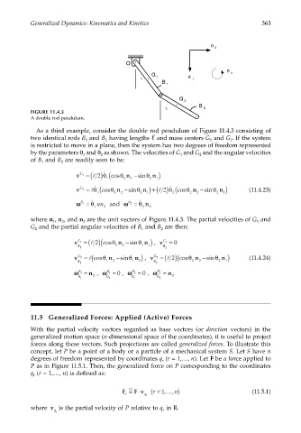
FIGURE 11.4.3
A double rod pendulum.
As a third example, consider the double rod pendulum of Figure 11.4.3 consisting of
two identical rods B and B having lengths and mass centers G and G . If the system
1 2 1 2
is restricted to move in a plane, then the system has two degrees of freedom represented
by the parameters θ and θ as shown. The velocities of G and G and the angular velocities
1 2 1 2
of B and B are readily seen to be:
1 2
v G 1 = (l 2) (cosθ ˙ θ n −sinθ n )
1 1 2 1 1
v G 2 = lθ ˙ 1 (cosθ 1 n −sinθ 1 n ) +(l 2) (cosθ ˙ 2 θ 2 n −sinθ 2 n ) (11.4.23)
2
1
2
1
ωω B 1 = θ ˙ un and ωω B 2 = θ ˙ n
1 3 2 3
where n , n , and n are the unit vectors of Figure 11.4.3. The partial velocities of G and
1 2 3 1
G and the partial angular velocities of B and B are then:
2 1 2
v G 1 = (l 2)( cosθ n − sinθ n , ) v G 1 = 0
˙ θ 1 1 2 1 1 ˙ θ 2
v G 2 = ( l cosθ n − sinθ n , ) v G 2 = (l 2)( cosθ n − sinθ n ) (11.4.24)
˙ θ 1 1 2 1 1 ˙ θ 2 2 2 2 1
ωω 1 B = n , ωω 1 B = 0 , ωω B 2 = 0 , ωω B 2 = n
˙ θ 1 3 ˙ θ 2 ˙ θ 1 ˙ θ 2 3

11.5 Generalized Forces: Applied (Active) Forces
With the partial velocity vectors regarded as base vectors (or direction vectors) in the
generalized motion space (n-dimensional space of the coordinates), it is useful to project
forces along these vectors. Such projections are called generalized forces. To illustrate this
concept, let P be a point of a body or a particle of a mechanical system S. Let S have n
degrees of freedom represented by coordinates q (r = 1,…, n). Let F be a force applied to
r
P as in Figure 11.5.1. Then, the generalized force on P corresponding to the coordinates
q (r = 1,…, n) is defined as:
r
⋅
D
F = F v ( r = …, n) (11.5.1)
1
,
r
˙
q r
where v is the partial velocity of P relative to q in R.
˙ q r r