Page 384 - Dynamics of Mechanical Systems

0593_C11_fm Page 365 Monday, May 6, 2002 2:59 PM

Generalized Dynamics: Kinematics and Kinetics 365

θ
k
B
P n θ
r i
i
Q

R
n r

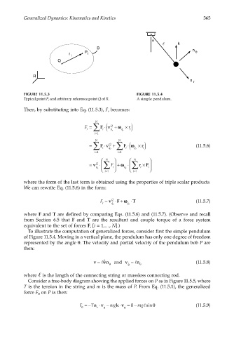
FIGURE 11.5.3 FIGURE 11.5.4
Typical point P i and arbitrary reference point Q of R. A simple pendulum.
Then, by substituting into Eq. (11.5.3), F becomes:
r

r ∑
F = N F i ( Q ˙ + ωω q r ˙ × r i)
⋅ v
q r
i=1
N
N
⋅ ωω
⋅
= ∑ Fv Q q r ∑ F i ( q r ˙ × r i) (11.5.6)
+
˙
i
i=1 i=1
 N   N 
i
= v Q ⋅ ∑ F + ωω ⋅ ∑ r × F i
i  =1  i  =1 
q r ˙ ˙ q r i
where the form of the last term is obtained using the properties of triple scalar products.
We can rewrite Eq. (11.5.6) in the form:
F = v Q ⋅ + ωω ⋅T (11.5.7)
F
r q r ˙ q r ˙
where F and T are defined by comparing Eqs. (11.5.6) and (11.5.7). (Observe and recall
from Section 6.5 that F and T are the resultant and couple torque of a force system
equivalent to the set of forces F [i = 1,…, N].)
i
To illustrate the computation of generalized forces, consider first the simple pendulum
of Figure 11.5.4. Moving in a vertical plane, the pendulum has only one degree of freedom
represented by the angle θ. The velocity and partial velocity of the pendulum bob P are
then:

v = lθ ˙ n θ and v = l n θ (11.5.8)
˙ θ

where is the length of the connecting string or massless connecting rod.
Consider a free-body diagram showing the applied forces on P as in Figure 11.5.5, where
T is the tension in the string and m is the mass of P. From Eq. (11.5.1), the generalized
force F on P is then:
θ
⋅
F =− Tnv θ ˙ − mg ⋅v θ ˙ = − mg sin θ (11.5.9)
l
k
0
θ
r