Page 387 - Dynamics of Mechanical Systems

0593_C11_fm Page 368 Monday, May 6, 2002 2:59 PM

368 Dynamics of Mechanical Systems

S
k
P(m) P S
1
n
h(q ,t)
r P
2

R R

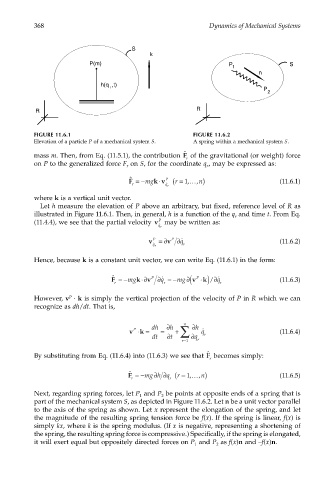
FIGURE 11.6.1 FIGURE 11.6.2
Elevation of a particle P of a mechanical system S. A spring within a mechanical system S.
ˆ
F
mass m. Then, from Eq. (11.5.1), the contribution of the gravitational (or weight) force
r
on P to the generalized force F on S, for the coordinate q , may be expressed as:
r
r
⋅
ˆ
F =− mg k v ( r = 1 ,… ,n) (11.6.1)
P
r ˙ q r
where k is a vertical unit vector.
Let h measure the elevation of P above an arbitrary, but fixed, reference level of R as
illustrated in Figure 11.6.1. Then, in general, h is a function of the q and time t. From Eq.
r
(11.4.4), we see that the partial velocity v P may be written as:
˙ q r
v =∂ v ∂ ˙ q (11.6.2)
P
P
˙ q r r
Hence, because k is a constant unit vector, we can write Eq. (11.6.1) in the form:
ˆ
F =− mg k⋅∂ v P ˙ q ∂ = − mg∂( v ⋅ k) / ˙ q∂ (11.6.3)
P
r r r
However, v · k is simply the vertical projection of the velocity of P in R which we can
P
recognize as dh/dt. That is,

n
v ⋅= dh = h ∂ + ∑ h ∂ q ˙ (11.6.4)
P
k
dt t ∂ q ∂ r
r=1 r
ˆ
By substituting from Eq. (11.6.4) into (11.6.3) we see that becomes simply:
F
r
ˆ
∂
∂
F =− mg h q ( r = 1 ,… ,n) (11.6.5)
r r
Next, regarding spring forces, let P and P be points at opposite ends of a spring that is
1
2
part of the mechanical system S, as depicted in Figure 11.6.2. Let n be a unit vector parallel
to the axis of the spring as shown. Let x represent the elongation of the spring, and let
the magnitude of the resulting spring tension force be f(x). If the spring is linear, f(x) is
simply kx, where k is the spring modulus. (If x is negative, representing a shortening of
the spring, the resulting spring force is compressive.) Specifically, if the spring is elongated,
it will exert equal but oppositely directed forces on P and P as f(x)n and –f(x)n.
2
1