Page 390 - Dynamics of Mechanical Systems

0593_C11_fm Page 371 Monday, May 6, 2002 2:59 PM

Generalized Dynamics: Kinematics and Kinetics 371

O y

O
O x
kx
1 k(x - x ) k(x - x )
3
2 1 1 2
G C
C C 3
1 2
C P P
1 1 2 P 3
C Mg
2
C mg k(x - x ) mg k(x - x ) mg kx
3
2
1
2
3 3
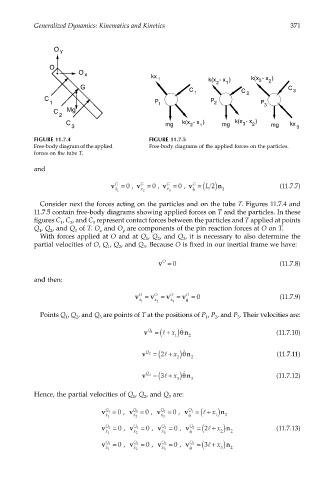
FIGURE 11.7.4 FIGURE 11.7.5
Free-body diagram of the applied Free-body diagrams of the applied forces on the particles.
forces on the tube T.
and
v = 0 , v = 0 , v = 0 , v = ( L 2) n (11.7.7)
G
G
G
G
˙ x 1 ˙ x 2 ˙ x 3 ˙ θ 2
Consider next the forces acting on the particles and on the tube T. Figures 11.7.4 and
11.7.5 contain free-body diagrams showing applied forces on T and the particles. In these
figures C , C , and C represent contact forces between the particles and T applied at points
2
3
1
Q , Q , and Q of T. O and O are components of the pin reaction forces at O on T.
3
y
1
2
x
With forces applied at O and at Q , Q , and Q , it is necessary to also determine the
2
3
1
partial velocities of O, Q , Q , and Q . Because O is fixed in our inertial frame we have:
3
1
2
O
v = 0 (11.7.8)
and then:
v = v = v = v = 0 (11.7.9)
O
O
O
O
˙ x 1 ˙ x 2 ˙ x 3 ˙ θ
Points Q , Q , and Q are points of T at the positions of P , P , and P . Their velocities are:
2
3
3
2
1
1
v Q 1 = (l + x )θ ˙ n (11.7.10)
1 2
l
v Q 2 = ( 2 + x )θ ˙ n (11.7.11)
2 2
= ( ˙
l
Q 3
v 3 + x )θ n (11.7.12)
3 3
Hence, the partial velocities of Q , Q , and Q are:
1
3
2
v Q 1 = 0 , v Q 1 = 0 , v Q 1 = 0 , v Q 1 = (l + x n )
˙ x 1 ˙ x 2 ˙ x 3 ˙ θ 1 2
2 +
v Q 2 = 0 , v Q 2 = 0 , v Q 2 = 0 , v Q 2 = ( l x n ) (11.7.13)
˙ x 1 ˙ x 2 ˙ x 3 ˙ θ 2 2
v Q 3 = 0 , v Q 3 = 0 , v Q 3 = 0 , v Q 3 = ( 3l + )n
l x
˙ x 1 ˙ x 2 ˙ x 3 ˙ θ 3 2