Page 393 - Dynamics of Mechanical Systems

0593_C11_fm Page 374 Monday, May 6, 2002 2:59 PM

374 Dynamics of Mechanical Systems

O + x 1 2 3 + x Reference Level
+ x 2
3
P 1
θ
P
2
P
3
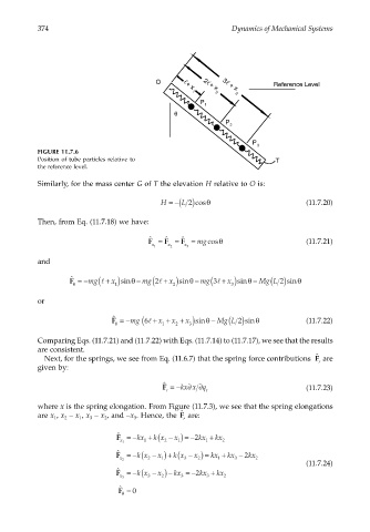
FIGURE 11.7.6
Position of tube particles relative to T
the reference level.

Similarly, for the mass center G of T the elevation H relative to O is:

H =−( ) 2 cosθ (11.7.20)
L

Then, from Eq. (11.7.18) we have:
ˆ
ˆ
ˆ
F = F = F = mg cosθ (11.7.21)
x 1 x 2 x 3
and
(
(
( )
ˆ
mg
x
x
x
F =− (l + ) sinθ − mg l2 + ) sinθ − mg l3 + ) sinθ − Mg L 2 sinθ
θ
1
2
3
or
(
( )
ˆ
x
F =−mg 6l + x 1 + x 2 + ) sinθ − Mg L 2 sinθ (11.7.22)
θ
3
Comparing Eqs. (11.7.21) and (11.7.22) with Eqs. (11.7.14) to (11.7.17), we see that the results
are consistent.
ˆ
Next, for the springs, we see from Eq. (11.6.7) that the spring force contributions F are
r
given by:
ˆ
∂
∂
F =− kx x q (11.7.23)
r r
where x is the spring elongation. From Figure (11.7.3), we see that the spring elongations
ˆ
are x , x – x , x – x , and –x . Hence, the are:
F
1 2 1 3 2 3 r
ˆ
F =− kx + ( x 2 kx + kx
k x − ) =−
x 1 1 2 1 1 2
k x − ) + (
F =− ( x k x − ) = kx + kx − 2 kx
ˆ
x
x 2 2 1 3 2 1 3 2
(11.7.24)
F =− ( x kx = − 2 kx + kx
ˆ
kx − ) −
x 3 3 2 3 3 2
ˆ
F = 0
θ