Page 79 - Dynamics of Mechanical Systems

0593_C03_fm Page 60 Monday, May 6, 2002 2:03 PM

60 Dynamics of Mechanical Systems

C
P

p
O

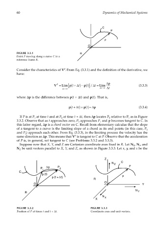
FIGURE 3.3.1 R
Point P moving along a curve C in a
reference frame R.

Consider the characteristics of V . From Eq. (3.3.1) and the definition of the derivative, we
P
have:

( [
P
V = Lim p t + ∆ t) − p t ()] ∆ t = Lim ∆ p (3.3.3)
/
0
∆ t→0 ∆ t→ ∆ t
where ∆p is the difference between p(t + ∆t) and p(t). That is,
(
p t + ∆ t) = p t () + ∆ p (3.3.4)

If P is at P at time t and at P at time t + ∆t, then ∆p locates P relative to P as in Figure
2
2
1
1
3.3.2. Observe that as t approaches zero, P approaches P and p becomes tangent to C. In
2
1
this latter regard, ∆p is a chord vector on C. Recall from elementary calculus that the slope
of a tangent to a curve is the limiting slope of a chord as its end points (in this case, P 1
and P ) approach each other. From Eq. (3.3.3), in the limiting process the velocity has the
2
P
same direction as ∆p. This means that V is tangent to C at P. Observe that the acceleration
of P is, in general, not tangent to C (see Problems 3.3.2 and 3.3.3).
Suppose now that X, Y, and Z are Cartesian coordinate axes fixed in R. Let N , N , and
Y
X
N be unit vectors parallel to X, Y, and Z, as shown in Figure 3.3.3. Let x, y, and z be the
Z
Z
N Z C
∆ p P P
P 2
1
C
p (t)
∆
p (t + t) p
R
O
O Y
N Y
R
N
X X
FIGURE 3.3.2 FIGURE 3.3.3
Position of P at times t and t + ∆t. Coordinate axes and unit vectors.