Page 84 - Dynamics of Mechanical Systems

0593_C03_fm Page 65 Monday, May 6, 2002 2:03 PM

Kinematics of a Particle 65

Z
Y
n
z
n
y
L
n
y n
Y
θ
n
x θ
X
X n L n x

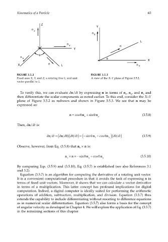
FIGURE 3.5.2 FIGURE 3.5.3
Fixed axes X, Y, and Z; a rotating line L; and unit A view of the X–Y plane of Figure 3.5.2.
vector parallel to L.

To verify this, we can evaluate dn/dt by expressing n in terms of n , n , and n and
y
z
x
then differentiate the scalar components as noted earlier. To this end, consider the X–Y
plane of Figure 3.5.2 as redrawn and shown in Figure 3.5.3. We see that n may be
expressed as:
n = cosθ n + sinθ n (3.5.8)
x y

Then, dn/dt is:

d dt = ( d d )( θ θ n + cos θ n y )( θ (3.5.9)
d dt)
n θ
d dt) =− ( sin
n
x
Observe, however, from Eq. (3.5.8) that n × n is:
z
n × n = −sinθ n + cosθ n (3.5.10)
z y y

By comparing Eqs. (3.5.9) and (3.5.10), Eq. (3.5.7) is established (see also References 3.1
and 3.2).
Equation (3.5.7) is an algorithm for computing the derivative of a rotating unit vector.
It is a convenient computational procedure in that it avoids the task of expressing n in
terms of fixed unit vectors. Moreover, it shows that we can calculate a vector derivative
in terms of a multiplication. This latter concept has profound implications for digital
computation. Indeed, a digital computer is ideally suited for performing the arithmetic
operations of addition, subtraction, multiplication, and division. Equation (3.5.7) thus
extends the capability to include differentiating without resorting to difference equations
as in numerical scalar differentiation. Equation (3.5.7) also forms a basis for the concept
of angular velocity as developed in Chapter 4. We will explore the application of Eq. (3.5.7)
in the remaining sections of this chapter.