Page 24 - Electric Drives and Electromechanical Systems

16 Electric Drives and Electromechanical Systems

though robotic manipulators are being considered, there is no difference between their
control and the control of the positioning axes of a CNC machine tool. The use of
polynomials to describe a trajectory is discussed in Section 2.5.
The trajectory that the end effector, and hence each joint, follows can be generated
from a knowledge of the robot’s kinematics, which defines the relationships between the
individual joints and the end effector’s position in Cartesian space. The solution of
the end effector position from the joint variables is termed forward kinematics, while the
determination of the joint variables from the robot’s position is termed inverse kine-
matics. To move the joints to the required position the actuators need to be driven under
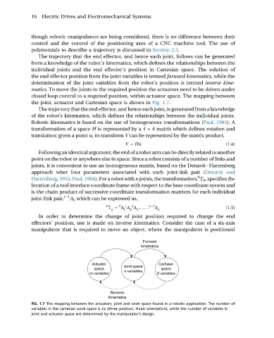
closed loop control to a required position, within actuator space. The mapping between
the joint, actuator and Cartesian space is shown in Fig. 1.7.
The trajectory that the end effector, and hence each joint, is generated from a knowledge
of the robot’s kinematics, which defines the relationships between the individual joints.
Robotic kinematics is based on the use of homogeneous transformations (Paul, 1984). A
transformation of a space H is represented by a 4 4 matrix which defines rotation and
translation; given a point u, its transform V can be represented by the matrix product,
V ¼ Hu (1.4)
Following anidentical argument, the end ofa robot arm can bedirectlyrelated toanother
point on the robot or anywhere else in space. Since a robot consists of a number of links and
joints, it is convenient to use an homogeneous matrix, based on the DenaviteHartenberg
approach wher four parameters associated with each joint-link pair (Denavit and
0
Hartenberg, 1955; Paul, 1984). For a robot with n joints, the transformation, T n ,specifies the
location of a tool interface coordinate frame with respect to the base coordinate system and
is the chain product of successive coordinate transformation matrices for each individual
joint-link pair, i 1 A i , which can be expressed as,
0 0 1 2 n 1
T ¼ A A A ..: A (1.5)
n i 2 3 n
In order to determine the change of joint position required to change the end
effectors’ position, use is made on inverse kinematics. Consider the case of a six-axis
manipulator that is required to move an object, where the manipulator is positioned

FIG. 1.7 The mapping between the actuators, joint and work space found in a robotic application. The number of
variables in the cartesian work space is six (three position, three orientation), while the number of variables in
joint and actuator space are determined by the manipulator’s design.