Page 105 - Electrical Properties of Materials

The density of states and the Fermi–Dirac distribution 87

1
F(E) =
k T ( ( exp (–E/k B T)
1 + exp E–E
F
1.0 B
1.0
T=0K Maxwell–Boltzmann
600K

0.5 6000K T=0K
Fermi–Dirac 600K
6000K

(a) E =2.5eV E (b) 2.5eV E
F
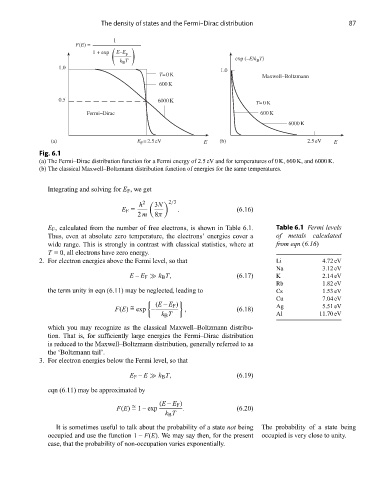
Fig. 6.1
(a) The Fermi–Dirac distribution function for a Fermi energy of 2.5 eV and for temperatures of 0 K, 600 K, and 6000 K.
(b) The classical Maxwell–Boltzmann distribution function of energies for the same temperatures.

Integrating and solving for E F , we get

h 2 3N 2/3
E F = . (6.16)
2 m 8π
E F , calculated from the number of free electrons, is shown in Table 6.1. Table 6.1 Fermi levels
Thus, even at absolute zero temperature, the electrons’ energies cover a of metals calculated
wide range. This is strongly in contrast with classical statistics, where at from eqn (6.16)
T = 0, all electrons have zero energy.
2. For electron energies above the Fermi level, so that Li 4.72 eV
Na 3.12 eV
E – E F k B T, (6.17) K 2.14 eV
Rb 1.82 eV
the term unity in eqn (6.11) may be neglected, leading to Cs 1.53 eV
Cu 7.04 eV

~ (E – E F ) Ag 5.51 eV
F(E) = exp – , (6.18)
k B T Al 11.70 eV
which you may recognize as the classical Maxwell–Boltzmann distribu-
tion. That is, for sufficiently large energies the Fermi–Dirac distribution
is reduced to the Maxwell–Boltzmann distribution, generally referred to as
the ‘Boltzmann tail’.
3. For electron energies below the Fermi level, so that

E F – E k B T, (6.19)
eqn (6.11) may be approximated by

(E – E F )
~
F(E) = 1–exp . (6.20)
k B T
It is sometimes useful to talk about the probability of a state not being The probability of a state being
occupied and use the function 1 – F(E). We may say then, for the present occupied is very close to unity.
case, that the probability of non-occupation varies exponentially.