Page 109 - Electrical Properties of Materials

Thermionic emission 91

term in the denominator. We are left then with some Gaussian functions, whose
integrals between ±∞ can be found in the better integral tables (you can derive
them for yourself if you are fond of doing integrals). This leads us to
4πmk B T E F /k B T –p /2 mk B T
2
N(p x )dp x = e e x d p x . (6.36)
h 3
Substituting eqn (6.36) into (6.30) and assuming that r(p x )= r is inde-
pendent of p x , which is not true but gives a good enough approximation, the
integration can be easily performed, leading to

2 –φ/k B T
J = A 0 (1 – r)T e , (6.37)
where
2
4πemk B 6 –2 –2
A 0 = =1.2 × 10 Am K . (6.38)
h 3
This is known as the Richardson (Nobel Prize, 1928) equation.
The most important factor in eqn (6.37) is exp(–φ/k B T), which is strongly
dependent both on temperature and on the actual value of the work function.
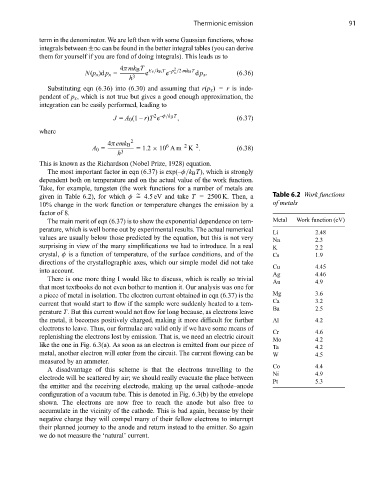
Take, for example, tungsten (the work functions for a number of metals are
~
given in Table 6.2), for which φ = 4.5 eV and take T = 2500 K. Then, a Table 6.2 Work functions
10% change in the work function or temperature changes the emission by a of metals
factor of 8.
The main merit of eqn (6.37) is to show the exponential dependence on tem- Metal Work function (eV)
perature, which is well borne out by experimental results. The actual numerical
Li 2.48
values are usually below those predicted by the equation, but this is not very Na 2.3
surprising in view of the many simplifications we had to introduce. In a real K 2.2
crystal, φ is a function of temperature, of the surface conditions, and of the Cs 1.9
directions of the crystallographic axes, which our simple model did not take
Cu 4.45
into account.
Ag 4.46
There is one more thing I would like to discuss, which is really so trivial
Au 4.9
that most textbooks do not even bother to mention it. Our analysis was one for
a piece of metal in isolation. The electron current obtained in eqn (6.37) is the Mg 3.6
Ca 3.2
current that would start to flow if the sample were suddenly heated to a tem-
Ba 2.5
perature T. But this current would not flow for long because, as electrons leave
the metal, it becomes positively charged, making it more difficult for further Al 4.2
electrons to leave. Thus, our formulae are valid only if we have some means of
Cr 4.6
replenishing the electrons lost by emission. That is, we need an electric circuit
Mo 4.2
like the one in Fig. 6.3(a). As soon as an electron is emitted from our piece of Ta 4.2
metal, another electron will enter from the circuit. The current flowing can be W 4.5
measured by an ammeter.
Co 4.4
A disadvantage of this scheme is that the electrons travelling to the
Ni 4.9
electrode will be scattered by air; we should really evacuate the place between
Pt 5.3
the emitter and the receiving electrode, making up the usual cathode–anode
configuration of a vacuum tube. This is denoted in Fig. 6.3(b) by the envelope
shown. The electrons are now free to reach the anode but also free to
accumulate in the vicinity of the cathode. This is bad again, because by their
negative charge they will compel many of their fellow electrons to interrupt
their planned journey to the anode and return instead to the emitter. So again
we do not measure the ‘natural’ current.