Page 111 - Electrical Properties of Materials

The Schottky effect 93

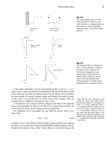
Fig. 6.4
The ‘image charge’ theorem. The
x x x x effect of a plane conductor on the
static field due to a charged particle is
equivalent to a second, oppositely
Conducting Remove plane charged, particle in the mirror image
plane add + charge position.

Energy x
0

Metal–vacuum B Image
interface field
x

A A
) a ( ) b (

Fig. 6.5
The Schottky effect. (a) Potential at
metal–vacuum interface. A denotes
Summarization the bottom of the potential well.
(b) Potential changed by image
charge field. (c) Potential due to
applied anode voltage in vacuum
region. (d) Total potential field
showing reduction in height of the
) c ( ) d ( potential barrier compared with (a).

In the above calculation, we took the potential energy as zero at x = ∞ to
agree with the usual conventions of electrostatics, but remember that our zero
a short while ago was that of a valence electron at rest. Hence, to be consistent,
we must redraw the energy diagram inside and outside the metal as shown
in Fig. 6.5(a). If we include now the effect of the mirror charges, then the ∗ Note that the curve between A and
∗
potential barrier modifies to that shown in Fig. 6.5(b). B does not satisfy eqn (6.40). This is
because the concept of a homogeneous
In the absence of an electric field this change in the shape of the potential
sheet is no longer applicable when x
barrier has practically no effect at all. But if we do have electric fields, the is comparable with the interatomic dis-
small correction due to mirror charges becomes significant. tance. The energy is, however, given for
For simplicity, let us investigate the case when the electric field is con- x = 0 (an electron resting on the sur-
face must have the same energy as an
stant. Then,
electron at rest inside the metal); so we
simply assume that eqn (6.40) is valid for
V(x)=–eE x, (6.41) x > x 0 and connect the points A and B by
a smooth line.
as shown in Fig. 6.5(c). If both an electric field is present and the mirror charges
are taken into account, then the potentials should be added, leading to the po-
tential barrier shown in Fig. 6.5(d). Clearly, there is a maximum that can be