Page 253 - Electrical Properties of Materials

The effective field 235

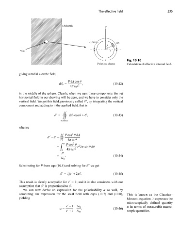
Dielectric

– Charge dA
θ

Void r

+ Fig. 10.10
Polarized charge Calculation of effective internal field.

giving a radial electric field,

P dA cos θ
dE r = , (10.42)
4π 0 r 2
in the middle of the sphere. Clearly, when we sum these components the net
horizontal field in our drawing will be zero, and we have to consider only the
vertical field. We get this field, previously called E , by integrating the vertical

component and adding to it the applied field, that is

£

E = dE r cos θ + E , (10.43)
surface
whence

P cos θ dA
£ 2

E – E =
4π 0 r 2
2
π P cos θ
2
= 2 r 2π sin θ dθ
0 4π 0 r
P
= . (10.44)
3 0

Substituting for P from eqn (10.5) and solving for E we get
1

E = ( +2)E . (10.45)
3
This result is clearly acceptable for = 1; and it is also consistent with our

assumption that E is proportional to E .
We can now derive an expression for the polarizability α as well, by
combining our expression for the local field with eqns (10.7) and (10.8), This is known as the Clausius–
yielding Mossotti equation. It expresses the
microscopically defined quantity

–1 3 0 α in terms of measurable macro-
α = · . (10.46)
scopic quantities.
+2 N m