Page 252 - Electrical Properties of Materials

234 Dielectric materials

Now suppose that a steady field is applied to align the molecules and then
switched off. The polarization and hence the internal field will diminish.
Following Debye, we shall assume that the field decays exponentially with a
time constant, τ, the characteristic relaxation time of the dipole moment of the
molecule,

P(t)= P 0 exp(–t/τ). (10.35)
You know that time variation and frequency spectrum are related by the
Fourier transform. In this particular case it happens to be true that the
relationship is

∞ iωt
K is a constant ensuring that f (ω) f (ω)= K P(t)e dt
0
has the right dimension.
KP 0
= , (10.36)
–iω +1/τ
using the condition (10.34) for the limit when ω = 0, we obtain
KP 0 τ = s – ∞ . (10.37)
s
Hence, eqn (10.33) becomes

s – ∞
∞ (ω)= ∞ + , (10.38)
–iωτ +1
which, after separation of the real and imaginary parts, reduces to

s – ∞

= ∞ + (10.39)
2 2
1+ ω τ
ωτ

= ( s – ∞ ). (10.40)
2 2
1+ ω τ
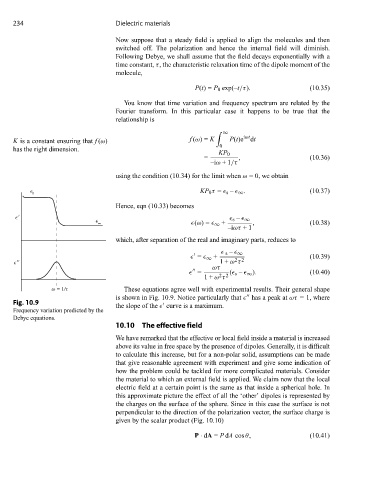
ω = 1/τ These equations agree well with experimental results. Their general shape

is shown in Fig. 10.9. Notice particularly that has a peak at ωτ = 1, where
Fig. 10.9
the slope of the curve is a maximum.
Frequency variation predicted by the
Debye equations.
10.10 The effective field
We have remarked that the effective or local field inside a material is increased
above its value in free space by the presence of dipoles. Generally, it is difficult
to calculate this increase, but for a non-polar solid, assumptions can be made
that give reasonable agreement with experiment and give some indication of
how the problem could be tackled for more complicated materials. Consider
the material to which an external field is applied. We claim now that the local
electric field at a certain point is the same as that inside a spherical hole. In
this approximate picture the effect of all the ‘other’ dipoles is represented by
the charges on the surface of the sphere. Since in this case the surface is not
perpendicular to the direction of the polarization vector, the surface charge is
given by the scalar product (Fig. 10.10)
P · dA = P dA cos θ, (10.41)