Page 255 - Electrical Properties of Materials

Acoustic waves 237

For ka 1, going over to the continuous case, the above equation
reduces to
1/2
β

ω = ka , (10.52)
m
whence a(β/m) 1/2 may be recognized as the velocity of acoustic waves, more
commonly known as the sound velocity.
We have found the dispersion equation for a solid built up from one kind of
atom. A somewhat more complicated case arises when there are two atoms in
a unit cell, with masses m 1 and m 2 . There are then two equations of motion,
one for each type of atom, as follows:
2

d x 2n
m 1 2 = β(x 2n+1 + x 2n–1 –2x 2n ), (10.53)
dt

2
d x 2n+1
m 2 2 = β(x 2n+2 + x 2n –2x 2n+1 ). (10.54)
dt
These equations can be solved with a moderate amount of sweat and toil but it
is really not worth the effort to do it here. The calculations are quite straight-
forward. They will be left as an exercise for the keener student. The solution is
obtained in the form,

ka 1/2
2
2
ω = β b 1 + b 2 ± (b 1 + b 2 ) –4b 1 b 2 sin 2 , (10.55)
2
where b 1 =1/m 1 and b 2 =1/m 2 .
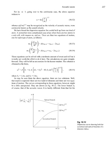
As may be seen from the above equation, there are two solutions. Well,
that much is expected: there are two kind of elements and there are two equa-
tions of motion. The curves corresponding to these equations, however, might
be a little unexpected. They are shown in Fig. 10.12. The lower branch is,
of course, that of the acoustic waves. It is hardly different from that for the

v

2b ( m 1 1 + m 1 2 ( 1/2 Optical branch

1/2
(2b/m 2 )
m >m (2b/m ) 1/2
1
1 2

Acoustical branch
Fig. 10.12
Dispersion curves showing both the
acoustical and optical branches of a
/ 2a k diatomic lattice.