Page 291 - Electrical Properties of Materials

Microscopic theory (quantum-mechanical) 273

Table 11.2 Hard magnetic materials

–1
Material H c (A m ) B r (T) (BH) max Jm –3
Carbon steel 0.9%C, 1% Mn 4.0 × 10 3 0.9 8 × 10 2
Alnico 5
8% Al, 24% Co, 3% Cu, 14% Ni 4.6 × 10 4 1.25 2 × 10 4
‘Ferroxdur’ (BaO)(Fe 2 O 3 ) 6 1.6 × 10 5 0.35 1.2 × 10 4
ESD Fe–Co 8.2 × 10 4 0.9 4 × 10 4
Alnico 9 1.3 × 10 5 1.05 10 5
SmCo 5 7 × 10 5 0.8 2 × 10 5
Nd 2 Fe 14 B 8.8 × 10 5 1.2 3 × 10 5

cannot easily be separated owing to their similar chemical properties. How- 1.4
ever, once the problem of separation was satisfactorily solved (early 1970s)
these magnets could be produced at an economic price. Their first champion
was the samarium–cobalt alloy SmCo 5 , produced by powdering and sintering. Sm(Co,Fe,Cu,Zr)
The next major advance owed its existence to political upheavals in Africa.
Uncertainties in the supply of cobalt, not to mention a five-fold price in-
crease, lent some urgency to the development of a cobalt-free permanent T
magnet. Experiments involving boron led to new (occasionally serendipitous) Nd–Fe–B
discoveries, culminating in the development of the Nd 2 Fe 14 B, which became
known as ‘neo’ magnets, referring not so much to their novelty (although new
they were) but to their neodymium content. They hold the current record of Sm Co 5
(BH) max = 400 kJ m –3 obtained under laboratory conditions. The commer- 0
–3
cially available value is about 300 kJ m , as may be seen in Table 11.2. They 800 400 0
have, though, the major disadvantage of a fairly low Curie temperature. Note kA m –1
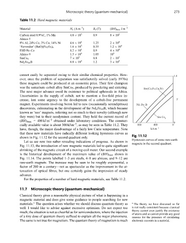
that these new materials have radically different looking hysteresis curves as
Fig. 11.12
shown in Fig. 11.12 for the second quadrant only.
Hysteresis curves of some rare-earth
Let us see now two rather revealing indications of progress. As shown in
magnets in the second quadrant.
Fig. 11.13, the introduction of new magnetic materials led to quite significant
shrinking of the magnetic circuit of a moving-coil meter. Our second example
is the historical development of the maximum value of (BH) max shown in
Fig. 11.14. The points labelled 1–3 are steels, 4–8 are alnicos, and 9–12 are
rare-earth magnets. The increase may be seen to be roughly exponential, a
factor of 200 in a century—not as spectacular as the improvement in the at-
tenuation of optical fibres, but one certainly gains the impression of steady
advance.
For the properties of a number of hard magnetic materials, see Table 11.2.

11.7 Microscopic theory (quantum-mechanical)

Classical theory gives a reasonable physical picture of what is happening in a
magnetic material and does give some guidance to people searching for new
materials. The question arises whether we should discuss quantum theory as ∗ Thetheorywehavediscussedsofar
∗
well. I would like to advise against excessive optimism. Do not expect too is not really consistent because classical
theory cannot even justify the existence
much; the situation is not as cheerful as for semiconductors, where the injection
of atoms and so cannot provide any good
of a tiny dose of quantum theory sufficed to explain all the major phenomena. reasons for the presence of circulating
The same is not true for magnetism. The quantum theory of magnetism is much electronic currents in a material.