Page 293 - Electrical Properties of Materials

Microscopic theory (quantum-mechanical) 275

moments, and there are quite a number of devices which need quantum theory
for their description. So let me describe the basic concepts.
First, we should ask how much of the previously outlined theory remains
valid in the quantum-mechanical formulation. Not a word of it! There is no
reason whatsoever why a classical argument (as, for example, the precession of
magnetic dipoles around the magnetic field) should hold water. When the res-
ulting formulae turn out to be identical (as, for example, for the paramagnetic ∗ This is sheer nonsense classically be-
susceptibility at normal temperatures), it is just a lucky coincidence. cause, according to classical mechanics,
once the angular momentum is known
So we have to start from scratch.
about three axes perpendicular to each
Let us first talk about the single electron of the hydrogen atom. As we men- other, it is known about any other axes
tioned before, the electron’s properties are determined by the four quantum (and it will not therefore take necessar-
numbers n, l, m l , and s, which have to obey certain relationships between ily integral multiples of a certain unit).
In quantum mechanics we may know the
themselves; as for example, that l must be an integer and may take values angular momentum about several axes
between 0 and n – 1. Any set of these four quantum numbers will uniquely de- but not simultaneously. Once the angu-
termine the properties of the electron. As far as the specific magnetic properties lar momentum is measured about one
of the electron are concerned, the following rules are relevant: axis, the measurement will alter the an-
gular momentum about some other axis
1. The total angular momentum is given by in an unpredictable way. If it were oth-
erwise, we would get into trouble with
the uncertainty relationship. Were we to
= { j( j +1)} 1/2 , (11.33) know the angular momentum in all dir-
ections, it would give us the plane of
1
where j = l + , that is a combination of the quantum numbers l and s. the electron’s orbit. Hence, we would
2 know the electron’s velocity in the dir-
2. The possible components of the angular momentum along any specified ection of the angular momentum vector
∗
direction are determined by the combination of m l (which may take on any (it would be zero), and also the position
integral value between –l and +l) and s, yielding (it would be in the plane perpendicular
to the angular momentum in line with
the proton). But this is forbidden by the
j, j –1, ... ,–j +1, –j. uncertainty principle, which says that it
is impossible to know both the velocity
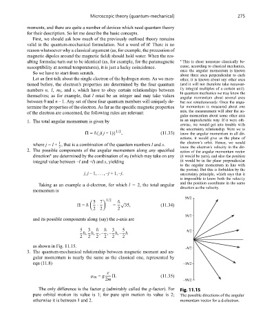
Taking as an example a d-electron, for which l = 2, the total angular and the position coordinate in the same
direction as the velocity.
momentum is
5h/2
5 7 √
1/2
= · = 35, (11.34)
2 2 2
3h/2
and its possible components along (say) the z-axis are
5 3 3 5 h/2
, , ,– ,– ,–
2 2 2 2 2 2
as shown in Fig. 11.15.
–h/2
3. The quantum-mechanical relationship between magnetic moment and an-
gular momentum is nearly the same as the classical one, represented by
eqn (11.8) –3h/2
e
μ m = g . (11.35)
2m –5h/2

The only difference is the factor g (admirably called the g-factor). For Fig. 11.15
pure orbital motion its value is 1; for pure spin motion its value is 2; The possible directions of the angular
otherwise it is between 1 and 2. momentum vector for a d-electron.