Page 155 - Electromagnetics

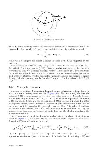
Figure 3.11: Multipole expansion.

where S ∞ is the bounding surface that recedes toward infinity to encompass all of space.
2
Because ∼ 1/r and D ∼ 1/r as r →∞, the integral over S ∞ tends to zero and
1
W = D(r) · E(r) dV. (3.88)
2
V ∞
Hence we may compute the assembly energy in terms of the fields supported by the
charge ρ.
It is significant that the assembly energy W is identical to the term within the time
derivative in Poynting’s theorem (2.299). Hence our earlier interpretation, that this term
represents the time-rate of change of energy “stored” in the electric field, has a firm basis.
Of course, the assembly energy is a static concept, and our generalization to dynamic
fields is purely intuitive. We also face similar questions regarding the meaning of energy
density, and whether energy can be “localized” in space. The discussions in § 2.9.5 still
apply.

3.2.6 Multipole expansion
Consider an arbitrary but spatially localized charge distribution of total charge Q
in an unbounded homogeneous medium (Figure 3.11). We have already obtained the
potential (3.61)of the source; as we move the observation point away, should decrease
in a manner roughly proportional to 1/r. The actual variation depends on the nature
of the charge distribution and can be complicated. Often this dependence is dominated
by a specific inverse power of distance for observation points far from the source, and we
can investigate it by expanding the potential in powers of 1/r. Although such multipole
expansions of the potential are rarely used to perform actual computations, they can
provide insight into both the behavior of static fields and the physical meaning of the
polarization vector P.
Let us place our origin of coordinates somewhere within the charge distribution, as
shown in Figure 3.11, and expand the Green’s function spatial dependence in a three-
dimensional Taylor series about the origin:

∞
1
1 n 1 1 1 1 2 1

= (r ·∇ ) = + (r ·∇ ) + (r ·∇ ) + ··· , (3.89)
R n! R r R 2 R

n=0 r =0 r =0 r =0

n

where R =|r − r |. Convergence occurs if |r| > |r |. In the notation (r ·∇ ) we interpret

a power on a derivative operator as the order of the derivative. Substituting (3.89)into
© 2001 by CRC Press LLC