Page 158 - Electromagnetics

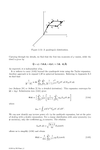
Figure 3.13: A quadrupole distribution.

Carrying through the details, we find that the first two moments of ρ vanish, while the
third is given by
¯
¯
Q = q[−3(d 1 d 2 + d 2 d 1 ) + 2(d 1 · d 2 )I].
As expected, it is independent of r 0 .
It is tedious to carry (3.92)beyond the quadrupole term using the Taylor expansion.
Another approach is to expand 1/R in spherical harmonics. Referring to Appendix E.3
we find that
n
∞
1

1 r n
∗

= 4π Y (θ ,φ )Y nm (θ, φ)
nm

|r − r | 2n + 1 r n+1
n=0 m=−n
(see Jackson [91] or Arfken [5] for a detailed derivation). This expansion converges for
|r| > |r m |. Substitution into (3.61)gives
n
∞
1
1 1
(r) = n+1 q nm Y nm (θ, φ) (3.94)
r 2n + 1
n=0 m=−n
where

n

∗

q nm = ρ(r )r Y (θ ,φ ) dV .
nm
V
We can now identify any inverse power of r in the multipole expansion, but at the price
of dealing with a double summation. For a charge distribution with axial symmetry (no
φ-variation), only the coefficient q n0 is nonzero. The relation

2n + 1
Y n0 (θ, φ) = P n (cos θ)
4π
allows us to simplify (3.94)and obtain
∞
1
1
(r) = q n P n (cos θ) (3.95)
4π r n+1
n=0
© 2001 by CRC Press LLC