Page 163 - Electromagnetics

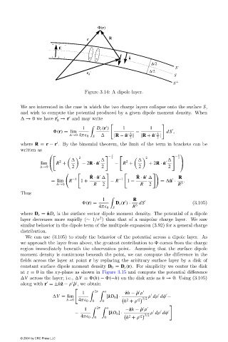
Figure 3.14: A dipole layer.

We are interested in the case in which the two charge layers collapse onto the surface S,
and wish to compute the potential produced by a given dipole moment density. When
→ 0 we have r → r and may write

0

1 D s (r ) 1 1

(r) = lim − dS ,
→0 4π 0 |R − ˆ n | |R + ˆ n |
S 2 2
where R = r − r . By the binomial theorem, the limit of the term in brackets can be

written as
 1 1 
− −
2 2 2 2
2
2
lim  R + − 2R · ˆ n − R + + 2R · ˆ n 
→0 2 2 2 2

ˆ
ˆ

R · ˆ n −1 R · ˆ n R

−1
= lim R 1 + − R 1 − = ˆ n · .

→0 R 2 R 2 R 3
Thus
1 R

(r) = D s (r ) · 3 dS (3.105)
4π 0 S R
where D s = ˆ nD s is the surface vector dipole moment density. The potential of a dipole
2
layer decreases more rapidly (∼ 1/r )than that of a unipolar charge layer. We saw
similar behavior in the dipole term of the multipole expansion (3.92)for a general charge
distribution.
We can use (3.105)to study the behavior of the potential across a dipole layer. As
we approach the layer from above, the greatest contribution to comes from the charge
region immediately beneath the observation point. Assuming that the surface dipole
moment density is continuous beneath the point, we can compute the difference in the
fields across the layer at point r by replacing the arbitrary surface layer by a disk of
constant surface dipole moment density D 0 = D s (r). For simplicity we center the disk
at z = 0 in the xy-plane as shown in Figure 3.15 and compute the potential difference
V across the layer; i.e., V = (h) − (−h) on the disk axis as h → 0. Using (3.105)
along with r =±hˆ z − ρ ˆρ , we obtain

1 2π a ˆ zh − ˆρ ρ

V = lim [ˆ zD 0 ] · 3/2 ρ dρ dφ −

2
h→0 4π 0 0 0 h + ρ 2

2π
a

1 −ˆ zh − ˆρ ρ

− ρ dρ dφ
[ˆ zD 0 ] ·
3/2
2
4π 0 0 0 h + ρ 2
© 2001 by CRC Press LLC