Page 166 - Electromagnetics

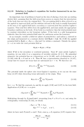
3.2.10 Solution to Laplace’s equation for bodies immersed in an im-
pressed field

An important class of problems is based on the idea of placing a body into an existing
electric field, assuming that the field arises from sources so remote that the introduction
of the body does not alter the original field. The pre-existing field is often referred to as
the applied or impressed field, and the solution external to the body is usually formulated
as the sum of the applied field and a secondary or scattered field that satisfies Laplace’s
equation. This total field differs from the applied field, and must satisfy the appropriate
boundary condition on the body. If the body is a conductor then the total potential must
be constant everywhere on the boundary surface. If the body is a solid homogeneous
dielectric then the total potential field must be continuous across the boundary.
As an example, consider a dielectric sphere of permittivity and radius a, centered at
the origin and immersed in a constant electric field E 0 (r) = E 0 ˆ z. By (3.30)the applied
potential field is 0 (r) =−E 0 z =−E 0 r cos θ (to within a constant). Outside the sphere
(r > a)we write the total potential field as

s
2 (r) = 0 (r) + (r)
s
s
where (r) is the secondary or scattered potential. Since must satisfy Laplace’s
equation, we can write it as a separation of variables solution (§ A.4). By azimuthal
symmetry the potential has an r-dependence as in (A.146), and a θ-dependence as in
s
(A.142)with B θ = 0 and m = 0.Thus has a representation identical to (A.147),
except that we cannot use terms that are unbounded as r →∞. We therefore use
∞
s
−(n+1)
(r,θ) = B n r P n (cos θ). (3.109)
n=0
The potential inside the sphere also obeys Laplace’s equation, so we can use the same
form (A.147)while discarding terms unbounded at the origin. Thus

∞

n
1 (r,θ) = A n r P n (cos θ) (3.110)
n=0
for r < a. To find the constants A n and B n we apply (3.36)and (3.37)to the total field.
Application of (3.36)at r = a gives

∞ ∞

−(n+1)
n
−E 0 a cos θ + B n a P n (cos θ) = A n a P n (cos θ).
n=0 n=0
Multiplying through by P m (cos θ) sin θ, integrating from θ = 0 to θ = π, and using the
orthogonality relationship (E.123), we obtain

−E 0 a + a −2 B 1 = A 1 a, (3.111)
n
B n a −(n+1) = A n a , n = 1, (3.112)
where we have used P 1 (cos θ) = cos θ. Next, since ρ s = 0, equation (3.37)requires that

∂ 1 (r) ∂ 2 (r)
1 = 2
∂r ∂r

© 2001 by CRC Press LLC