Page 164 - Electromagnetics

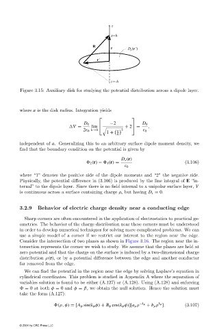
Figure 3.15: Auxiliary disk for studying the potential distribution across a dipole layer.

where a is the disk radius. Integration yields

 
D 0 −2 D 0
V = lim  + 2  = ,
a 2
2 0 h→0 0
1 +
h
independent of a. Generalizing this to an arbitrary surface dipole moment density, we
find that the boundary condition on the potential is given by

D s (r)
2 (r) − 1 (r) = (3.106)
0
where “1” denotes the positive side of the dipole moments and “2” the negative side.
Physically, the potential difference in (3.106)is produced by the line integral of E “in-
ternal” to the dipole layer. Since there is no field internal to a unipolar surface layer, V
is continuous across a surface containing charge ρ s but having D s = 0.

3.2.9 Behavior of electric charge density near a conducting edge

Sharp corners are often encountered in the application of electrostatics to practical ge-
ometries. The behavior of the charge distribution near these corners must be understood
in order to develop numerical techniques for solving more complicated problems. We can
use a simple model of a corner if we restrict our interest to the region near the edge.
Consider the intersection of two planes as shown in Figure 3.16. The region near the in-
tersection represents the corner we wish to study. We assume that the planes are held at
zero potential and that the charge on the surface is induced by a two-dimensional charge
distribution ρ(r), or by a potential difference between the edge and another conductor
far removed from the edge.
We can find the potential in the region near the edge by solving Laplace’s equation in
cylindrical coordinates. This problem is studied in Appendix A where the separation of
variables solution is found to be either (A.127)or (A.128). Using (A.128)and enforcing
= 0 at both φ = 0 and φ = β, we obtain the null solution. Hence the solution must
take the form (A.127):

k φ
(ρ, φ) = [A φ sin(k φ φ) + B φ cos(k φ φ)][a ρ ρ −k φ + b ρ ρ ]. (3.107)

© 2001 by CRC Press LLC