Page 209 - Electromagnetics

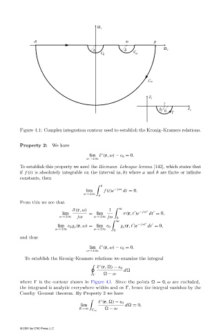
Figure 4.1: Complex integration contour used to establish the Kronig–Kramers relations.

Property 2: We have
c
lim ˜ (r,ω) − 0 = 0.
ω→±∞
To establish this property we need the Riemann–Lebesgue lemma [142], which states that
if f (t) is absolutely integrable on the interval (a, b) where a and b are finite or infinite
constants, then
b

lim f (t)e − jωt dt = 0.
ω→±∞
a
From this we see that
˜ σ(r,ω) 1 ∞ − jωt
lim = lim σ(r, t )e dt = 0,

ω→±∞ jω ω→±∞ jω 0
∞

χ e (r, t )e − jωt dt = 0,
lim 0 χ e (r,ω) = lim 0
ω→±∞ ω→±∞
0
and thus
c
lim ˜ (r,ω) − 0 = 0.
ω→±∞
To establish the Kronig–Kramers relations we examine the integral
c
˜ (r, ) − 0
d
− ω

where is the contour shown in Figure 4.l. Since the points = 0, ω are excluded,
the integrand is analytic everywhere within and on , hence the integral vanishes by the
Cauchy–Goursat theorem. By Property 2 we have
c
˜ (r, ) − 0
lim d = 0,
R→∞ − ω
C ∞
© 2001 by CRC Press LLC