Page 210 - Electromagnetics

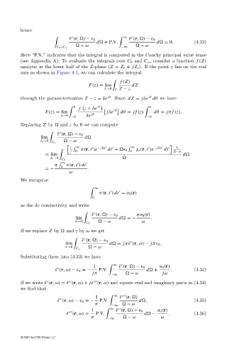
hence
c ∞ c
˜ (r, ) − 0 ˜ (r, ) − 0
d + P.V. d = 0. (4.33)
− ω − ω
C 0 +C ω −∞
Here “P.V.” indicates that the integral is computed in the Cauchy principal value sense
(see Appendix A). To evaluate the integrals over C 0 and C ω , consider a function f (Z)
analytic in the lower half of the Z-plane (Z = Z r + jZ i ). If the point z lies on the real
axis as shown in Figure 4.1, we can calculate the integral

f (Z)
F(z) = lim dZ
δ→0 Z − z
jθ
jθ
through the parameterization Z − z = δe . Since dZ = jδe dθ we have

0 f z + δe jθ 0
F(z) = lim jδe jθ dθ = jf (z) dθ = jπ f (z).
δ→0 −π δe jθ −π
Replacing Z by and z by 0 we can compute

c
˜ (r, ) − 0
lim d
→0 − ω
C 0

1 ∞ − j t ∞ − j t 1

σ(r, t )e dt + 0 χ e (r, t )e dt
j 0 0 −ω
= lim d
→0
C 0
∞
π 0 σ(r, t ) dt

=− .
ω
We recognize

∞

σ(r, t ) dt = σ 0 (r)

0
as the dc conductivity and write
c
˜ (r, ) − 0 πσ 0 (r)
lim d =− .
→0 − ω ω
C 0
If we replace Z by and z by ω we get
c
˜ (r, ) − 0 c
lim d = jπ ˜ (r,ω) − jπ 0 .
δ→0 − ω
C ω
Substituting these into (4.33) we have
c
1 ∞ ˜ (r, ) − 0 σ 0 (r)
c
˜ (r,ω) − 0 =− P.V. d + . (4.34)
jπ −∞ − ω jω
c
If we write ˜ (r,ω) = ˜ (r,ω) + j ˜ (r,ω) and equate real and imaginary parts in (4.34)
c
c
we find that
c
1 ∞ ˜ (r, )
c
˜ (r,ω) − 0 =− P.V. d , (4.35)
π −∞ − ω
1 ∞ ˜ (r, ) − 0 σ 0 (r)
c
c
˜ (r,ω) = P.V. d − . (4.36)
π − ω ω
−∞
© 2001 by CRC Press LLC