Page 119 -

R

V S V
C C

L

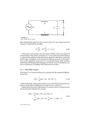
FIGURE 4.5
RLC circuit with ac source.
RLC Circuit: Referring to the RLC circuit in Figure 4.5, the voltage across the
capacitor is described by the ODE:

2
dV dV
LC 2 c + RC C + V = V t() (4.29)
C
s
dt dt
Numerically solving these and other types of ODEs will be the subject of
the remainder of this section. In Section 4.7.1, we consider first-order iterators
to represent the different-order derivatives, apply this algorithm to solve the
above types of problems, and conclude by pointing out some of the limita-
tions of this algorithm. In Section 4.7.2, we discuss higher-order iterators,
particularly the Runge-Kutta technique. In Section 4.7.3, we familiarize our-
selves with the use of standard MATLAB solvers for ODEs.

4.7.1 First-Order Iterator

In Section 4.5, we found an improved expression for the numerical differen-
tiator, D(k):

Dk() = 2 [ yk( ) − yk( − 1 )] − D k( − 1 ) (4.16)
t ∆

which functionally corresponded to the inverse of the Trapezoid rule for inte-
gration. (Note that the independent variable here is t, and not x.)
Applying this first-order differentiator in cascade leads to an expression for
the second-order differentiator, namely:

2
Dk2() = [ Dk( ) − Dk 1( − )] − D k2( − 1)
t ∆
(4.30)
= 4 [ yk( ) − yk 1( − )] − 4 Dk 1( − ) − D k2( − 1)
(∆ t) 2 t ∆

© 2001 by CRC Press LLC