Page 139 -

but, because s is a non-negative number smaller than 1, the right-hand-side of
the inequality in Eq. (5.9) can be made, for large enough value of m, arbitrarily
small, and the above iterative procedure does indeed converge to a fixed point.

Example 5.1
Find the zero of the function:

y = x – sin(x) – 1 (5.10)

Solution: At the zero, the iterative form can be written as:

x(k) = sin(x(k – 1)) + 1 (5.11)

The contraction property, required for the application of this method, is valid
in this case because the difference between two sines is always smaller than
the difference between their arguments. The fixed point can then be obtained
by the following MATLAB program:

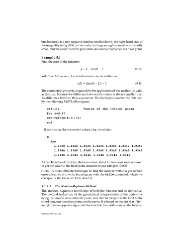
x(1)=1; %value of the initial guess
for k=2:20
x(k)=sin(x(k-1))+1;
end

If we display the successive values of x, we obtain:

x
Ans
1.0000 1.8415 1.9636 1.9238 1.9383 1.9332 1.9350
1.9344 1.9346 1.9345 1.9346 1.9346 1.9346 1.9346
1.9346 1.9346 1.9346 1.9346 1.9346 1.9346

As can be noticed from the above printout, about 11 iterations were required
to get the value of the fixed point accurate to one part per 10,000.
NOTE A more efficient technique to find the answer within a proscribed
error tolerance is to write the program with the while command, where we
can specify the tolerance level desired.

5.1.2.2 The Newton-Raphson Method
This method requires a knowledge of both the function and its derivative.
The method makes use of the geometrical interpretation of the derivative
being the tangent at a particular point, and that the tangent is the limit of the
chord between two close points on the curve. It is based on the fact that if f(x )
1
and f(x ) have opposite signs and the function f is continuous on the interval
2
© 2001 by CRC Press LLC