Page 137 -

4. Use the crosshair of the ginput command to read the coordinates
of the intersection.

In problems where we desire to find the zeros of a function that depends
on two input variables, we follow (conceptually) the same steps above, but
use 3-D graphics.

In-Class Exercises
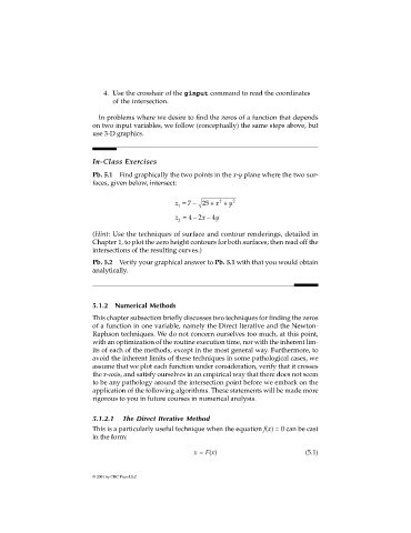
Pb. 5.1 Find graphically the two points in the x-y plane where the two sur-
faces, given below, intersect:

z =− 25 + x + y 2
2
7
1
z =− x − 4 y
42
2
(Hint: Use the techniques of surface and contour renderings, detailed in
Chapter 1, to plot the zero height contours for both surfaces; then read off the
intersections of the resulting curves.)
Pb. 5.2 Verify your graphical answer to Pb. 5.1 with that you would obtain
analytically.

5.1.2 Numerical Methods
This chapter subsection briefly discusses two techniques for finding the zeros
of a function in one variable, namely the Direct Iterative and the Newton-
Raphson techniques. We do not concern ourselves too much, at this point,
with an optimization of the routine execution time, nor with the inherent lim-
its of each of the methods, except in the most general way. Furthermore, to
avoid the inherent limits of these techniques in some pathological cases, we
assume that we plot each function under consideration, verify that it crosses
the x-axis, and satisfy ourselves in an empirical way that there does not seem
to be any pathology around the intersection point before we embark on the
application of the following algorithms. These statements will be made more
rigorous to you in future courses in numerical analysis.

5.1.2.1 The Direct Iterative Method
This is a particularly useful technique when the equation f(x) = 0 can be cast
in the form:

x = F(x) (5.1)

© 2001 by CRC Press LLC