Page 247 -

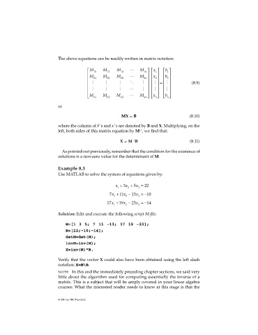
The above equations can be readily written in matrix notation:

 M 11 M 12 M 13 L M   x  b  
1
n
1
1
     
 M 21 M 22 M 23 L M 2 n   x 2   b 2 
 M M M O M   M  =   (8.9)
M
     
M
 M M M L M   M   
  M n1 M n2 M n3 L M   x   b  
n
nn 
n
or
MX = B (8.10)
where the column of b’ s and x’ s are denoted by B and X. Multiplying, on the
–1
left, both sides of this matrix equation by M , we find that:
–1
X = M B (8.11)
As pointed out previously, remember that the condition for the existence of
solutions is a non-zero value for the determinant of M.

Example 8.3
Use MATLAB to solve the system of equations given by:

x + 3 x + 5 x = 22
1 2 3
7 x + 11 x − 13 x = − 10
1 2 3
17 x + 19 x − 23 x = − 14
1 2 3

Solution: Edit and execute the following script M-file:

M=[1 3 5; 7 11 -13; 17 19 -23];
B=[22;-10;-14];
detM=det(M);
invM=inv(M);
X=inv(M)*B.

Verify that the vector X could also have been obtained using the left slash
notation: X=M\B.
NOTE In this and the immediately preceding chapter sections, we said very
little about the algorithm used for computing essentially the inverse of a
matrix. This is a subject that will be amply covered in your linear algebra
courses. What the interested reader needs to know at this stage is that the

© 2001 by CRC Press LLC