Page 259 -

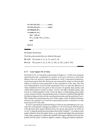
X=[x1;x2;x3;.......;xn];
Y=[y1;y2;y3;.......;yn];
n=length(X);
V=ones(n,n);
for j=2:n
V(:,j)=X.*V(:,j-1);
end

A=V\Y

In-Class Exercises
Find the polynomials that are defined through:

Pb. 8.10 The points (1, 5), (2, 11), and (3, 19).
Pb. 8.11 The points (1, 8), (2, 39), (3, 130), (4, 341), and (5, 756).

8.7.7 Least Square Fit of Data
In Section 8.7.6, we found the polynomial of degree (n – 1) that was uniquely
determined by the coordinates of n points on its curve. However, when data
fitting is the tool used by experimentalists to verify a theoretical prediction,
many more points than the minimum are measured in order to minimize the
effects of random errors generated in the acquisition of the data. But this
over-determination in the system parameters faces us with the dilemma of
what confidence level one gives to the accuracy of specific data points, and
which data points to accept or reject. A priori, one takes all data points, and
resorts to a determination of the vector A whose corresponding polynomial
comes closest to all the experimental points. Closeness is defined through the
Euclidean distance between the experimental points and the predicted curve.
This method for minimizing the sum of the square of the Euclidean distance
between the optimal curve and the experimental points is referred to as the
least-square fit of the data.
To have a geometrical understanding of what we are attempting to do, con-
sider the conceptually analogous problem in 3-D of having to find the plane
with the least total square distance from five given data points. So what do
we do? Using the projection procedure derived in Chapter 7, we deduce each
point’s distance from the plane; then we go ahead and adjust the parameters
of the plane equation to obtain the smallest total square distance between the
points and the plane. In linear algebra courses, using generalized optimiza-

© 2001 by CRC Press LLC