Page 260 -

tion techniques, you will be shown that the best fit to A (i.e., the one called
least-square fit) is given (using the rotation of the previous subsection) by:

T
–1
T
A = (V V) V Y (8.26)
N
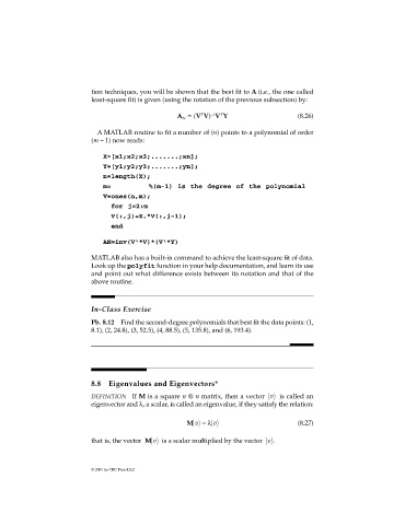
A MATLAB routine to fit a number of (n) points to a polynomial of order
(m – 1) now reads:
X=[x1;x2;x3;.......;xn];
Y=[y1;y2;y3;.......;yn];
n=length(X);
m= %(m-1) is the degree of the polynomial
V=ones(n,m);
for j=2:m
V(:,j)=X.*V(:,j-1);
end

AN=inv(V'*V)*(V'*Y)

MATLAB also has a built-in command to achieve the least-square fit of data.
Look up the polyfit function in your help documentation, and learn its use
and point out what difference exists between its notation and that of the
above routine.

In-Class Exercise
Pb. 8.12 Find the second-degree polynomials that best fit the data points: (1,
8.1), (2, 24.8), (3, 52.5), (4, 88.5), (5, 135.8), and (6, 193.4).

8.8 Eigenvalues and Eigenvectors*
DEFINITION If M is a square n ⊗ n matrix, then a vector v is called an
eigenvector and λ, a scalar, is called an eigenvalue, if they satisfy the relation:

M v =λ v (8.27)

that is, the vector M v is a scalar multiplied by the vector v .

© 2001 by CRC Press LLC