Page 265 -

8.9 The Cayley-Hamilton and Other Analytical Techniques*
In Section 8.8, we presented the general techniques for computing the eigen-
values and eigenvectors of square matrices, and showed their power in solv-
ing systems of coupled linear differential equations. In this section, we add to
our analytical tools arsenal some techniques that are particularly powerful
when elegant solutions are desired in low-dimensional problems. We start
with the Cayley-Hamilton theorem.

8.9.1 Cayley-Hamilton Theorem
The matrix M satisfies its own characteristic equation.
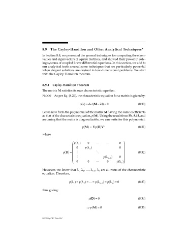
PROOF As per Eq. (8.29), the characteristic equation for a matrix is given by:

p( )λ = det(M − λI ) = 0 (8.30)

Let us now form the polynomial of the matrix M having the same coefficients
as that of the characteristic equation, p(M). Using the result from Pb. 8.15, and
assuming that the matix is diagonalizable, we can write for this polynomial:

p(M) = Vp(D)V –1 (8.31)

where

 p(λ 1 ) 0 L L 0 
 0 p(λ ) 0 
 2 
p D () =  M O  (8.32)
 M p(λ 
  n−1 ) 0  
 0 0 L 0 p(λ n  )

However, we know that λ , λ , …, λ , λ are all roots of the characteristic
1
2
n
n–1
equation. Therefore,
p(λ ) = p(λ ) = … = p(λ ) = p(λ ) = 0 (8.33)
1 2 n 1− n
thus giving:

p()D = 0 (8.34)

⇒ p(M ) = 0 (8.35)

© 2001 by CRC Press LLC