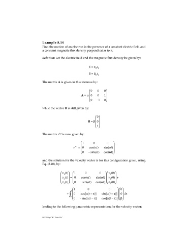
Page 271 -

Example 8.14
Find the motion of an electron in the presence of a constant electric field and
a constant magnetic flux density perpendicular to it.

Solution: Let the electric field and the magnetic flux density be given by:

r
E = E ê
03
r
B = B ê
01
The matrix A is given in this instance by:

0 0  0
 
A = α 0 0 1
 
0 −1  0

while the vector B is still given by:

  0
 
B = β 0
 
  1

At
The matrix e is now given by:

1 0 0 

e A t = 0 cos(α t) sin(α t) 
 
0 − sin(α t) cos(α t  )

and the solution for the velocity vector is for this configuration given, using
Eq. (8.40), by:

 vt ()  1 0 0   v 0 ()
1
1

 vt () =  0 cos(α t) sin(α t)   v 0 () +

  2       2  
 vt () 0  − sin(α t) cos(α t)  v 0 ()
3
3
 1 0 0    0
t
+  ∫  0 cos[α t ( − τ )] sin[α t ( − τ )]   
0 dτ
0   
0  − sin[α t ( − τ )] cos[α t ( − τ)])]   β
leading to the following parametric representation for the velocity vector:
© 2001 by CRC Press LLC