Page 172 - Elements of Distribution Theory

P1: JZP
052184472Xc05 CUNY148/Severini May 24, 2005 17:53

158 Parametric Families of Distributions

n
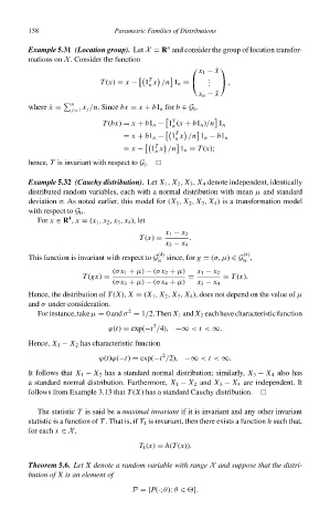
Example 5.31 (Location group). Let X = R and consider the group of location transfor-
mations on X. Consider the function
x 1 − ¯ x
 
T
.
T (x) = x − 1 x /n 1 n =  .  ,
n .
x n − ¯ x
n
where ¯ x = x j /n. Since bx = x + b1 n for b ∈ G l ,
j=1
T

T (bx) = x + b1 n − 1 (x + b1 n )/n 1 n
n
T

= x + b1 n − 1 x /n 1 n − b1 n
n
T
= x − 1 x /n 1 n = T (x);
n
hence, T is invariant with respect to G l .
Example 5.32 (Cauchy distribution). Let X 1 , X 2 , X 3 , X 4 denote independent, identically
distributed random variables, each with a normal distribution with mean µ and standard
deviation σ.As noted earlier, this model for (X 1 , X 2 , X 3 , X 4 )isa transformation model
with respect to G ls .
4
For x ∈ R , x = (x 1 , x 2 , x 3 , x 4 ), let
x 1 − x 2
T (x) = .
x 3 − x 4
(4) (4)
This function is invariant with respect to G since, for g = (σ, µ) ∈ G ,
ls ls
(σ x 1 + µ) − (σ x 2 + µ) x 1 − x 2
T (gx) = = = T (x).
(σ x 3 + µ) − (σ x 4 + µ) x 3 − x 4
Hence, the distribution of T (X), X = (X 1 , X 2 , X 3 , X 4 ), does not depend on the value of µ
and σ under consideration.
2
For instance, take µ = 0 and σ = 1/2. Then X 1 and X 2 each have characteristic function
2
ϕ(t) = exp(−t /4), −∞ < t < ∞.
Hence, X 1 − X 2 has characteristic function
2
ϕ(t)ϕ(−t) = exp(−t /2), −∞ < t < ∞.
It follows that X 1 − X 2 has a standard normal distribution; similarly, X 3 − X 4 also has
a standard normal distribution. Furthermore, X 1 − X 2 and X 3 − X 4 are independent. It
follows from Example 3.13 that T (X) has a standard Cauchy distribution.

The statistic T is said be a maximal invariant if it is invariant and any other invariant
statistic is a function of T . That is, if T 1 is invariant, then there exists a function h such that,
for each x ∈ X,

T 1 (x) = h(T (x)).

Theorem 5.6. Let X denote a random variable with range X and suppose that the distri-
bution of X is an element of
P ={P(·; θ): θ ∈ }.