Page 187 - Elements of Distribution Theory

P1: JZP
052184472Xc06 CUNY148/Severini May 24, 2005 2:41

6.2 Discrete Time Stationary Processes 173

= 0 = 0.5

x t x t
− −
− −

t t
= −0.5 = 0.9

x t x t
− −
− −

t t
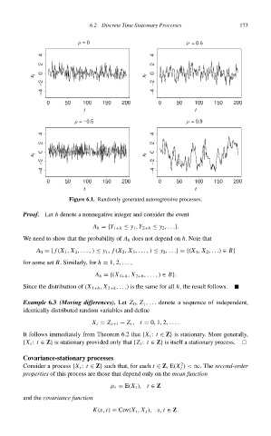
Figure 6.1. Randomly generated autoregressive processes.

Proof. Let h denote a nonnegative integer and consider the event
A h ={Y 1+h ≤ y 1 , Y 2+h ≤ y 2 ,...}.

We need to show that the probability of A h does not depend on h. Note that
A 0 ={ f (X 1 , X 2 ,..., ) ≤ y 1 , f (X 2 , X 3 ,..., ) ≤ y 2 ,...}={(X 1 , X 2 ,...) ∈ B}
for some set B. Similarly, for h = 1, 2,...,

A h ={(X 1+h , X 2+h ,..., ) ∈ B}.
Since the distribution of (X 1+h , X 2+h ,...)is the same for all h, the result follows.

Example 6.3 (Moving differences). Let Z 0 , Z 1 ,... denote a sequence of independent,
identically distributed random variables and define
X t = Z t+1 − Z t , t = 0, 1, 2,....
It follows immediately from Theorem 6.2 that {X t : t ∈ Z} is stationary. More generally,
{X t : t ∈ Z} is stationary provided only that {Z t : t ∈ Z} is itself a stationary process.

Covariance-stationary processes
2
Consider a process {X t : t ∈ Z} such that, for each t ∈ Z,E(X ) < ∞. The second-order
t
properties of this process are those that depend only on the mean function
µ t = E(X t ), t ∈ Z
and the covariance function

K(s, t) = Cov(X t , X s ), s, t ∈ Z.