Page 234 - Elements of Distribution Theory

P1: JZX
052184472Xc07 CUNY148/Severini May 24, 2005 3:59

220 Distribution Theory for Functions of Random Variables

Itfollowsthat X (m) ,themthorderstatistic,hasadiscretedistributionwithfrequencyfunction

p (m) (t)
m n+k−m
n t m−k n − m + k j tj (t+1)(n−m+k− j)
= [1 − (1 − θ) ] θ (1 − θ) (1 − θ)
m − k j
k=1 j=k
m n+k−m j
n t m−k (t+1)(n−m+k) n − m + k θ
= [1 − (1 − θ) ] (1 − θ) .
m − k j 1 − θ
k=1 j=k
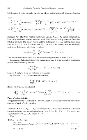
Example 7.24 (Uniform random variables). Let X 1 , X 2 ,..., X n denote independent,
identically distributed random variables, each distributed according to the uniform dis-
tribution on (0, 1). The density function of this distribution is I {0<t<1} and the distribution
function is t,0 < t < 1. It follows that X (m) , the mth order statistic, has an absolutely
continuous distribution with density function

n − 1 m−1 n−m

p (m) (t) = n t (1 − t) , 0 < t < 1.
m − 1
This distribution is known as a beta distribution with parameters m and n − m + 1.
In general, a beta distribution with parameters α and β is an absolutely continuous
distribution with density function
(α + β) α−1 β−1
x (1 − x) , 0 < x < 1;
(α) (β)
here α> 0 and β> 0 are not restricted to be integers.
By Theorem 7.6, X (m) has distribution function
n
n i n−i
t (1 − t) , 0 < t < 1.
i
i=m
Hence, we obtain the useful result
t n
n − 1 m−1 n−m n i n−i
n u (1 − u) du = t (1 − t) , 0 < t < 1.
m − 1 0 i=m i
Pairs of order statistics
An approach similiar to that used in Theorem 7.6 can be used to determine the distribution
function of a pair of order statistics.

Theorem 7.8. Let X 1 , X 2 ,..., X n denote independent, identically distributed, real-valued
random variables each with distribution function F. Let X (1) , X (2) ,..., X (n) denote the
order statistics of X 1 ,..., X n and let m < r.
Then
Pr(X (m) ≤ s, X (r) ≤ t)
n n−i n i i− j n−i− j

i=m F(s) [F(t) − F(s)] [1 − F(t)] if s < t
 j=max(0,r−i) i, j,n−i− j
= .
Pr(X (r) ≤ t) if s ≥ t
