Page 233 - Elements of Distribution Theory

P1: JZX
052184472Xc07 CUNY148/Severini May 24, 2005 3:59

7.5 Order Statistics 219

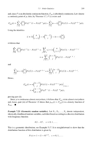
and, since F is an absolutely continuous function, F (m) is absolutely continuous. Let t denote

a continuity point of p; then, by Theorem 1.7, F (t)exists and
n n
n i−1 n−i n i n−1−i

F (m) (t) = i F(t) (1 − F(t)) p(t) − (n − i) F(t) (1 − F(t)) p(t).
i=m i i=m i
Using the identities

n n − 1 n

(i + 1) = n = (n − i) ,
i + 1 i i
it follows that
m n−1
n i−1 n−i n j n−1− j
i F(t) (1 − F(t)) = ( j + 1) F(t) (1 − F(t))
i j + 1
i=m j=m−1
n−1
n − 1 j n−1− j
= n F(t) (1 − F(t))
j
j=m−1
and

n n−1
n i n−1−i n − 1 i n−1−i
(n − i) F(t) (1 − F(t)) = n F(t) (1 − F(t)) .
i i
i=m i=m
Hence,

n − 1 j n−1− j
F (t) = n F(t) (1 − F(t))
(m) p(t)
j j=m−1
n − 1 m−1 n−m

= n F(t) (1 − F(t)) p(t),
m − 1
proving part (ii).
Since p is continuous almost everywhere, it follows that F exists almost everywhere
(m)
and, hence, part (iii) of Theorem 1.9 shows that p (m) (t) = F (t)isa density function of
(m)
X (m) .

Example 7.23 (Geometric random variables). Let X 1 , X 2 ,..., X n denote independent,
identically distributed random variables, each distributed according to a discrete distribution
with frequency function

x
θ(1 − θ) , x = 0, 1,....
This is a geometric distribution; see Example 5.17. It is straightforward to show that the
distribution function of this distribution is given by

F(x) = 1 − (1 − θ) x+1 , x = 0, 1,....