Page 228 - Elements of Distribution Theory

P1: JZX
052184472Xc07 CUNY148/Severini May 24, 2005 3:59

214 Distribution Theory for Functions of Random Variables

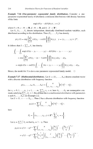
Example 7.16 (One-parameter exponential family distribution). Consider a one-
parameter exponential family of absolutely continuous distributions with density functions
of the form

exp{c(θ)y − d(θ)}h(y), y ∈ Y
+
where θ ∈ , c : → R, d : → R, and h : Y → R .
Let Y 1 , Y 2 ,..., Y n denote independent, identically distributed random variables, each
distributed according to this distribution. Then (Y 1 ,..., Y n ) has density

n n
n
p(y; θ) = exp c(θ)y j − nd(θ) h(y j ), y = (y 1 ,..., y n ) ∈ Y .
j=1 j=1
n
It follows that S = Y j has density
j=1

··· exp{c(θ)(s − y 2 − ... − y n ) − d(θ)}h(s − y 2 −· · · − y n )
Y Y

n n

× exp c(θ)y j − (n − 1) d(θ) h(y j ) dy 2 ··· dy n
j=2 j=2
n

= exp{c(θ)s − nd(θ)} ··· h(s − y 2 −· · · − y n ) h(y j ) dy 2 ··· dy n .
Y Y j=2
Hence, the model for S is also a one-parameter exponential family model.
Example 7.17 (Multinomial distribution). Let X = (X 1 ,..., X m ) denote a random vector
with a discrete distribution with frequency function
n

x 1 x 2
x m
p(x 1 ,..., x m ; θ 1 ,...,θ m ) = θ θ ··· θ ,
1 2 m
x 1 , x 2 ,... x m
m
for x j = 0, 1,..., n, j = 1,..., m, j=1 x j = n; here θ 1 ,...,θ m are nonnegative con-
m

stants satisfying θ j = 1. Recall that this is a multinomial distribution with parameters
j=1
n and (θ 1 ,...,θ m ); see Example 2.2.
Let S = X 1 +· · · + X m−1 . Then S has a discrete distribution with frequency function

n
x m
x 1 x 2
p S (s) = θ θ ··· θ ;
1 2 m
x 1 ,..., x m
X s
here
m−1

m
X s = (x 1 ,..., x m−1 ) ∈ Z : x j = s .
j=1
m−1

Let η = θ j so that θ m = 1 − η. Then
j=1
n θ 1 θ m−1
x 1 x m−1

n−s
s
p S (s) = η (1 − η) ···
x 1 , x 2 ,..., x m η η
X s
n

s θ 1 x 1 θ m−1 x m−1
n−s
s
= η (1 − η) x 1 ,...,x m ··· .
s

x 1 ,..., x m η η
X s x 1 ,...,x m